Global oceanic barrier model on the sphere
Alba Fuster-Alonso1 Elias T Krainski2 Haavard Rue3 Finn Lindgren4
Source:vignettes/web/barrier_global.Rmd
barrier_global.RmdIntroduction
In this tutorial, we illustrate the implementation of the barrier model proposed in Bakka et al. (2019) in the sphere. It considers the problem of modeling over a spatial domain, taking into account physical barriers and the spherical shape of the Earth. Since we are working on the global oceans, continents can be considered as physical barriers, and this aspect has to be taken into account in the modeling. When using a barrier model, the range is not only determined by the distance to points. If there is a barrier between two points, the range should decrease quickly, and the correlation over the barrier should approach zero. Additionally, the Earth’s spherical shape is a crucial factor in this particular case, as considering a planar approximation can bias the results when working on a global scale. Therefore, this tutorial is developed using a projection onto a sphere. We are using the new implementation of the INLA package.
## Load required libraries
library(rnaturalearth)
library(sf)
library(ggplot2)
library(INLA)
library(INLAspacetime)
library(inlabru)
library(ggOceanMaps)
library(s2)
library(DOYPAColors)
library(ggpubr)
Define barriers
Our initial step is to define the barriers in the model. As we aim to model an oceanic variable, it is essential to treat all continents as barriers. To accomplish this, we must establish specific parameters, including the mesh resolution, maximum edge length of the mesh, and define a distance and a buffer to simplify certain country polygons. If we increase the mesh resolution, the computational time will also increase.
## Mesh resolution (bigger number increases the resolution)
sresol <- 30

## This resolution will gives the approximate maximum edge length (in km)
max_edge <- 36080.2 * 0.2 / sresol
units(max_edge) <- "km"

## Set a minimum distance to be used for simplification of polygons
dist_simplify <- 20
units(dist_simplify) <- "km"

## Set a buffer distance to be added to certain polygons
bufferdist <- max_edge / 2
Subsequently, we use the ne_countries function from the rnaturalearth package to download data for all countries, employing the Mollweide projection. We specify that we want an object class of Simple Features (sf) for ease in conducting spatial operations.
## Download country boundaries data at a medium scale
world_ll <- ne_countries(scale = "medium", returnclass = "sf")

## Retrieve the coordinate reference system (CRS) of the downloaded data
crs_ll <- st_crs(world_ll)

## Define Mollweide projection
crs_vis <- st_crs("+proj=moll +units=km +units=km")

## Transform the country boundaries data to the Mollweide projection
world_mll <- st_transform(st_geometry(world_ll), crs_vis)
We now create a function to define a bounding box around the earth in the latlong projection. This will be used later.
## function to create a Earth polygon
Earth_poly <- function(resol = 100) {
    st_sfc(st_multipolygon(
        list(st_polygon(list(cbind(
            long = c(
                seq(-1, 1, length.out = resol * 2 + 1), rep(1, resol + 1),
                seq(1, -1, length.out = resol * 2 + 1), rep(-1, resol + 1)
            ) * (180 - 1e-5),
            lat = c(
                rep(1, resol * 2 + 1), seq(1, -1, length.out = resol + 1),
                rep(-1, resol * 2 + 1), seq(-1, 1, length.out = resol + 1)
            ) * (90 - 1e-5)
        ))))), crs = "+proj=longlat +datum=WGS84 +no_defs +ellps=WGS84 +towgs84=0,0,0")
}
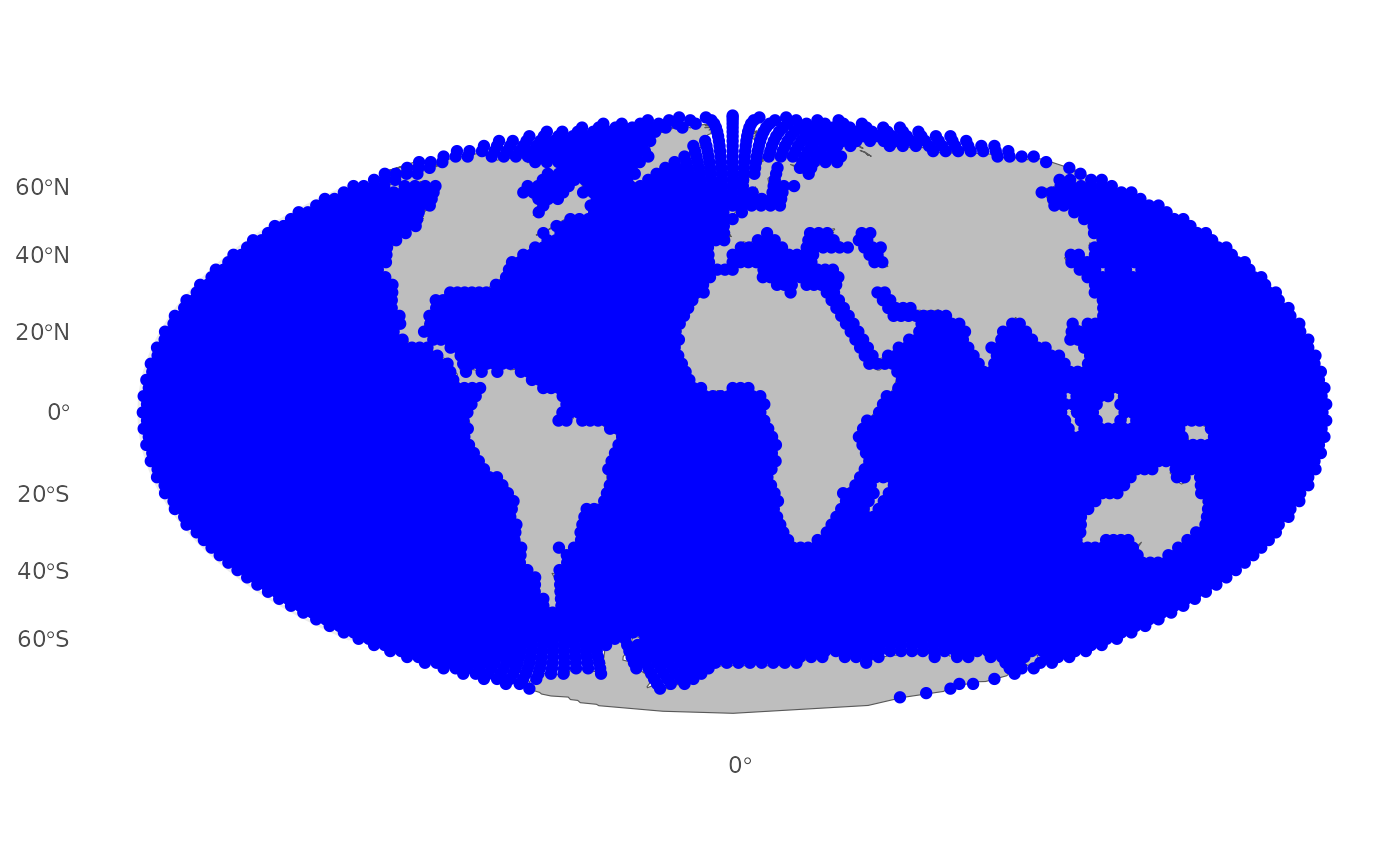
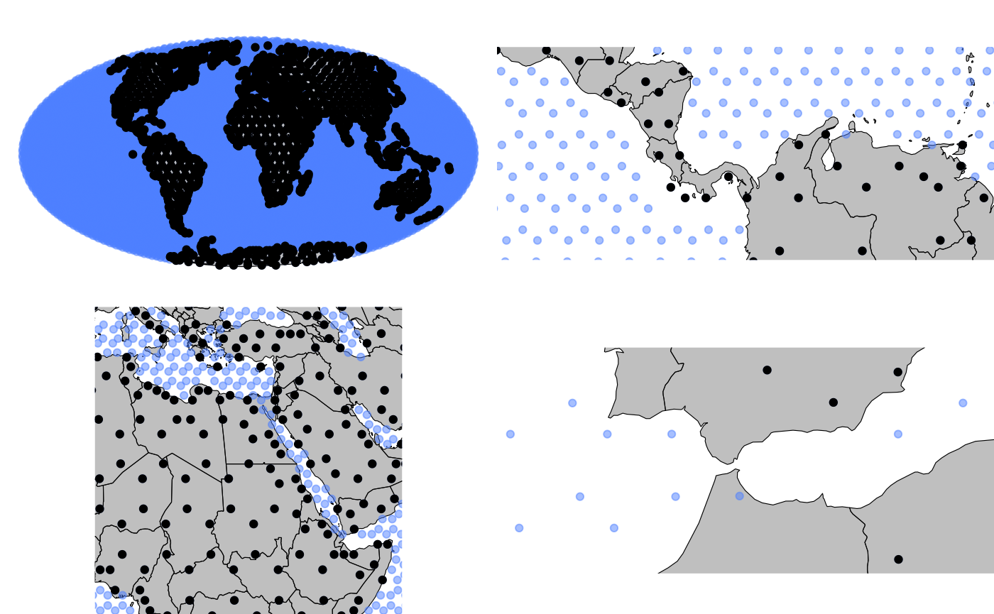
We also need to prepare a grid for projecting the effects of the model, considering the Mollweide projection and the spherical shape of the Earth. To accomplish this, we have implemented a function called grid_create. This function creates a grid of points within a specified boundary that do not intersect with a given barrier. The barrier can be either a Simple Features (sf) or Simple Features Collection (sfc) object representing a geographic region, and the boundary can be specified by either providing a boundary object or numeric limits for x and y axes.
## Function to create the grid for projection while considering the barrier
grid_create <- function(barrier, resol = 50) {
  if (!inherits(barrier, c("sf", "sfc"))) {
    stop("barrier must be sf or sfc objects.")
  }
  Ell <- Earth_poly(resol = 100)
  if (st_crs(Ell) != st_crs(barrier)) {
    Ell_transformed <- st_transform(Ell, st_crs(barrier))
  } else {
    Ell_transformed <- Ell
  }
  grid_0 <- st_as_sf(
    expand.grid(x = seq(from = min(st_coordinates(Ell_transformed)[,1]),
                        to = max(st_coordinates(Ell_transformed)[,1]),
                        by = resol),
                y = seq(from = min(st_coordinates(Ell_transformed)[,2]),
                        to = max(st_coordinates(Ell_transformed)[,2]),
                        by = resol)),
    coords = 1:2, crs = st_crs(barrier))
  ig_0 <- which(sapply(st_intersects(grid_0, Ell_transformed), length) > 0)
  ig_sel <- setdiff(ig_0,
                   which(sapply(st_intersects(grid_0, barrier), length) > 0)
  )
  grid_mll <- grid_0[ig_sel, ]
  return(grid_mll)
}

## Grid in Mollweide
mgrid <- grid_create(barrier = world_mll)

## Grid in latlong
grid_ll <- st_transform(mgrid, crs = crs_ll)

## Transform to the sphere
mgrid_sph <- fm_transform(
    mgrid,
    crs = fm_crs("sphere")
)
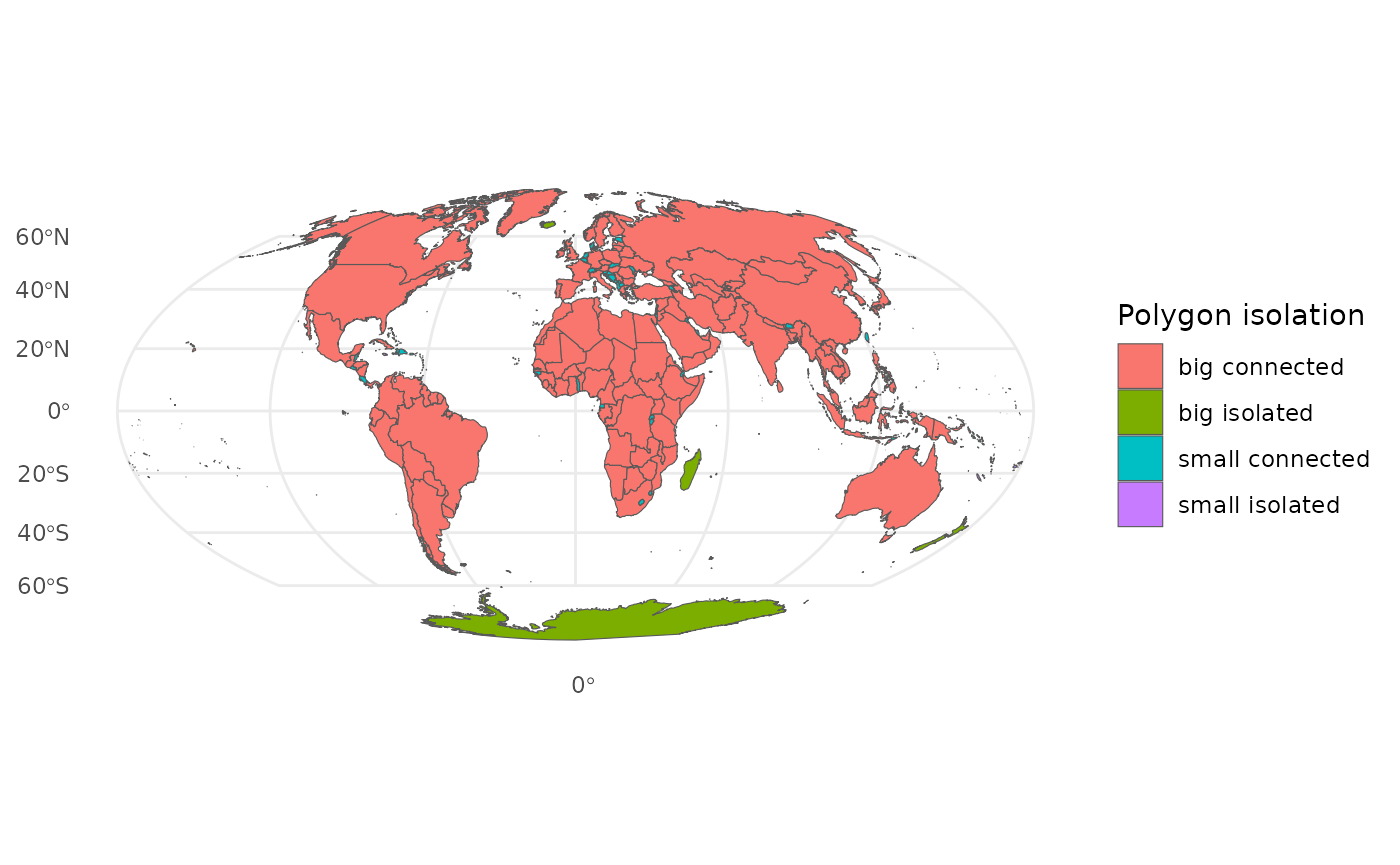
At this point, we will modify some of the barrier polygons to enhance realism and facilitate computation. First, we will calculate the area of each polygon downloaded earlier and if they are isolated or not. This is to identify small and isolated islands that may not be relevant to our model, and we should exclude them from the barrier.
## Compute the area of each polygon
world_area <- st_area(world_mll)

## Extract the neighbor list from this map (consider neighbor if any coordinate within the buffer distance)
nb <- spdep:::poly2nb(
                pl = world_mll,
                snap = as.numeric(bufferdist))

## Number of neighbors
nn <- spdep::card(nb)

## Identify small multipolygons (area smaller than square of the approximated maximum length of the edges in the modeling domain)
wpolyclass <- paste(ifelse(sqrt(world_area) > max_edge, "big", "small"),
                    ifelse(nn>0, "connected", "isolated"))
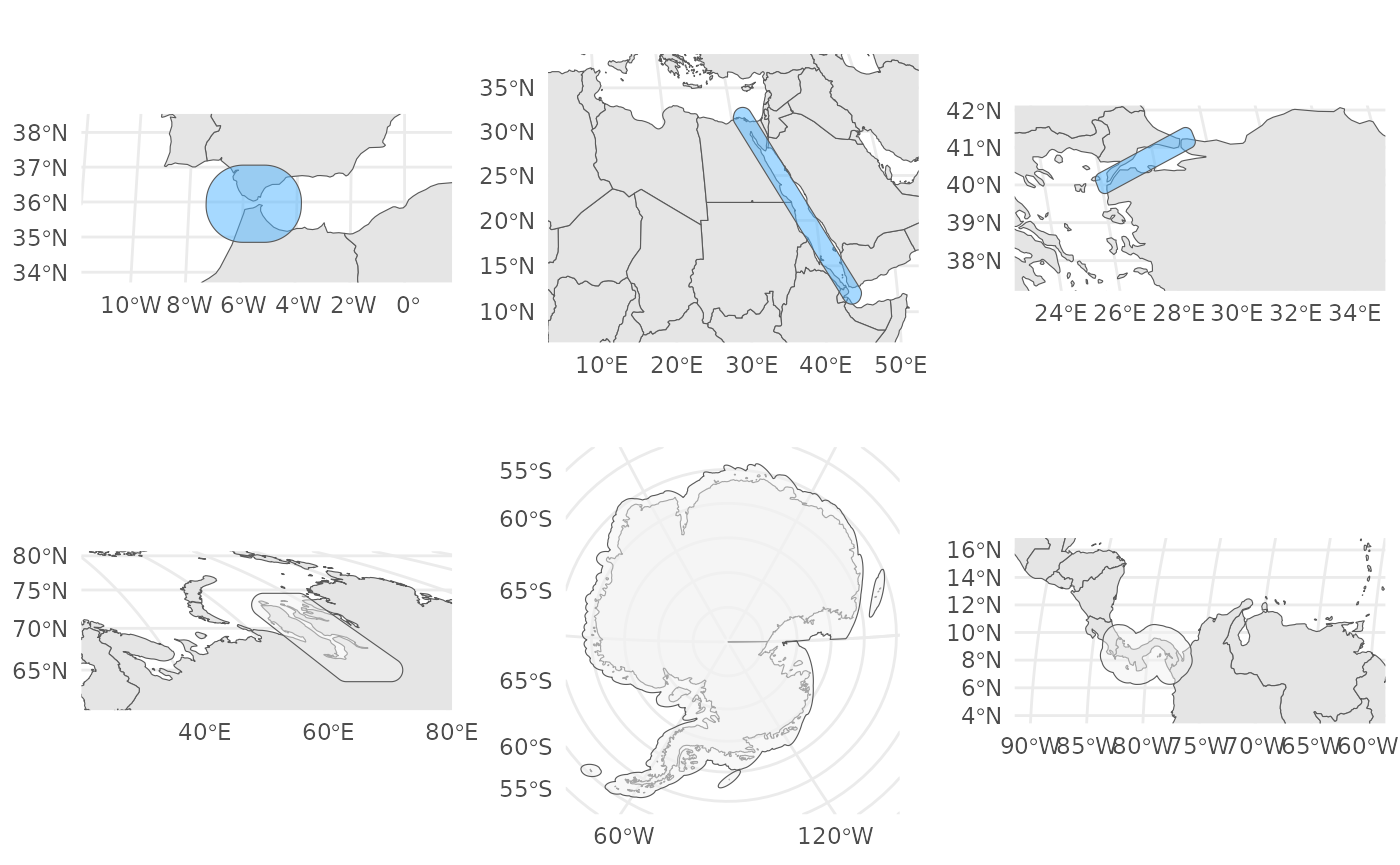
Moreover, we will give the option for expanding some straits, such as the Suez Canal or the Strait of Gibraltar to minimize correlation near the borders.
## Enlarge Suez canal
## Define the coordinates for the Suez canal polygon
suez_ll <- matrix(
    c(31.6, 31.7, 43.9, 43.8, 31.6,
      31.5, 31.7, 12.0, 11.8, 31.5),
    ncol = 2, byrow = FALSE)

## Create a Simple Features (sf) polygon for the Suez canal
suez_ll <- sf::st_sfc(
    sf::st_polygon(
        list(suez_ll)
    ), crs = crs_ll
)

## Transform the Suez canal polygon and create a buffer
suez_mll <- st_buffer(
    st_transform(suez_ll, crs_vis),
    dist = bufferdist
)

## Enlarge strait of Gibraltar
## Define the coordinates for the Strait of Gibraltar polygon
gibra_ll <- matrix(
    c(-6.0, -5.2, -5.2, -6.0, -6.0,
      36.0, 36.0, 35.9, 35.9, 36.0),
    ncol = 2, byrow = FALSE)

## Create a Simple Features (sf) polygon for the Strait of Gibraltar
gibra_ll <- sf::st_sfc(
    sf::st_polygon(
        list(gibra_ll)
    ), crs = crs_ll
)

## Transform the Strait of Gibraltar polygon and create a buffer
gibra_mll <- st_buffer(
    st_transform(gibra_ll, crs_vis),
    dist = bufferdist
)

## Enlarge Turkish straits
## Define the coordinates for the Turkish straits polygon
turk_ll <- matrix(
  c(26.1, 39.95,
    29.35, 41.15,
    29.3, 41.35,
    26.05, 40.15,
    26.1, 39.95),
  ncol = 2, byrow = TRUE
)

## Create a Simple Features (sf) polygon for the  Turkish straits
turk_ll <- sf::st_sfc(
    sf::st_polygon(
        list(turk_ll)
    ), crs = crs_ll
)

## Transform the Turkish straits polygon and create a buffer
turk_mll <- st_buffer(
    st_transform(turk_ll, crs_vis),
    dist = bufferdist/6
)
After identifying the area and isolation of the polygons, we will remove those polygons from the barrier that are considered isolated and small.
### Remove small and isolated polygons
world_barrier_initial <- st_difference(
    world_mll[wpolyclass != "small isolated"],
    st_union(c(suez_mll, gibra_mll, turk_mll))
    )
Likewise, we plan to incorporate buffers around specific regions of the world. For example, we want to account for the closure of the Panama Canal, consider the ice cover of Antarctica, and include a buffer around the Gulf of Ob to facilitate the simulation.
## Panama country polygon retrieval and buffer creation
panm_ll <- ne_countries(country = "panama", scale = "medium", returnclass = "sf")
panm_mll <- st_buffer(
    st_transform(st_geometry(panm_ll), crs_vis),
    dist = bufferdist)

## Define the coordinates for the Gulf of Ob polygon
gulf_ll <- matrix(
  c(70, 78, 78, 70, 70,
    65, 65, 73, 73, 65),
  ncol = 2, byrow = FALSE)

## Create a Simple Features (sf) polygon for the Gulf of Ob
gulf_ll <- sf::st_sfc(
  sf::st_polygon(
    list(gulf_ll)
  ), crs = crs_ll
)

## Transform the Gulf of Ob polygon and create a buffer
gulf_mll <- st_buffer(
  st_transform(gulf_ll, crs_vis),
  dist = bufferdist)

## Download Antarctica polygon
antar_ll <- ne_countries(country = "Antarctica", scale = "medium", returnclass = "sf")

## Include a buffer
antar_mll <- st_buffer(
  st_transform(st_geometry(antar_ll), crs_vis),
  dist = bufferdist)
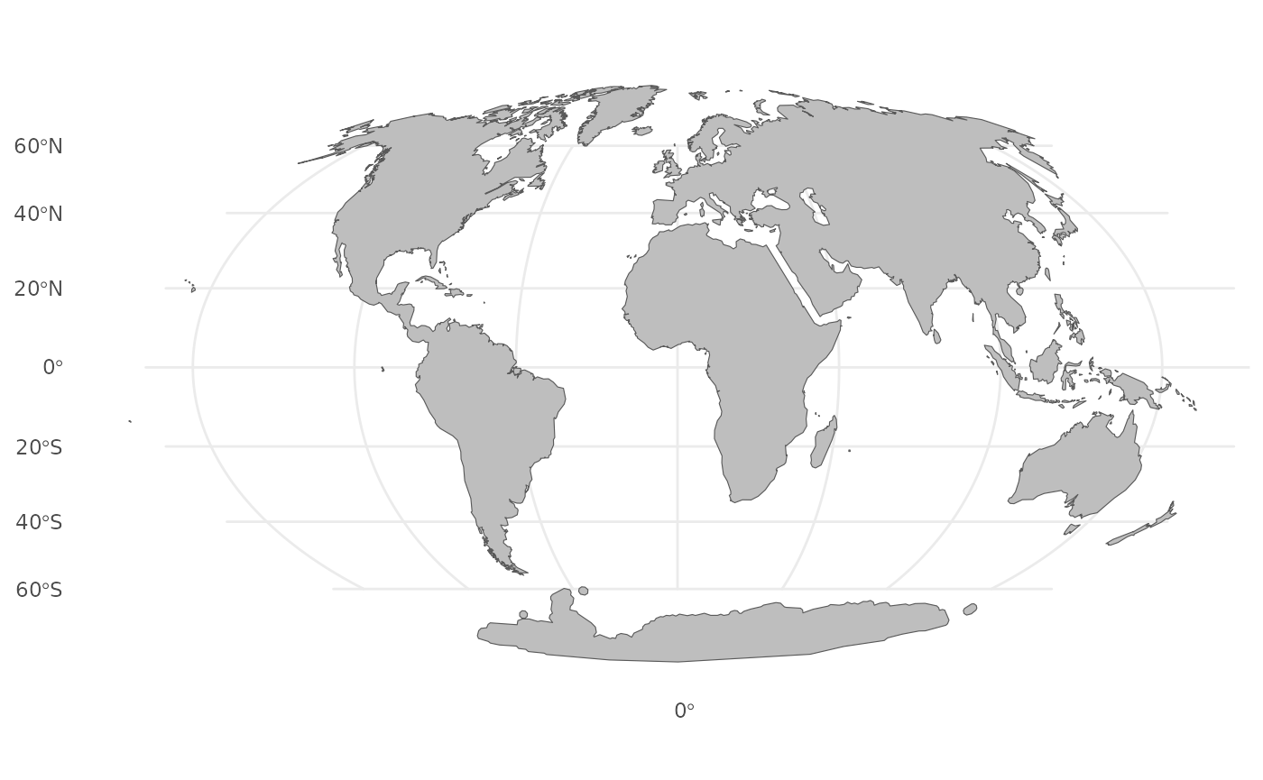
Once the specific polygons have been modified, we can proceed to integrate them with our multipolygon of world countries. We also use the st_simplify function to simplify the borders of the polygons while preserving the topology of the domain.
## Buffer world land
world_lnd <- st_union(c(world_barrier_initial, panm_mll, gulf_mll, antar_mll))

## World land excluding the Suez canal, Turkish straits, and Gibraltar strait
world_dff <- st_difference(
    x = world_lnd,
    y = st_union(c(suez_mll, gibra_mll, turk_mll))
)

## World land without modifications for visualization
world_union <- st_union(world_mll)

## Join and simplify the boundary of the barrier domain so that very detailed parts would be smoothed out
world_barrier <- st_simplify(
    world_dff,
    preserveTopology = FALSE,
    dTolerance = dist_simplify)
Classifying polygon areas
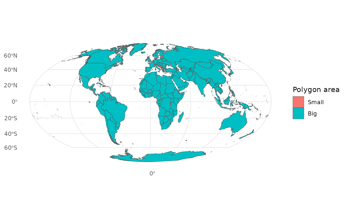
Classify polygons based on size, where TRUE indicates a large polygon, and FALSE indicates a small polygon.
Mesh Creation
The barrier model proposed by Bakka et al. (2019), involves a triangulation method. Therefore, we are going to consider an underlying random field over the whole sphere; and this random field will be discretized using the mesh, defining a precision matrix for the distribution at the mesh nodes. In order to work more efficiently, we will simulate higher-resolution points outside the barrier using the fmesher_globe_points function. This allows us to utilize these initial points to reduce the number of nodes inside the barrier. Consequently, this will improve computation speed without compromising the results of the model. It’s crucial to note that the mesh is designed with consideration for a sphere (fm_transform), allowing us to work in three dimensions.
## Create a initial set of points over the globe considering the desired resolution
reg.glob.pts <- fmesher_globe_points(
    globe = sresol ## subdivision resolution for a semi-regular spherical triangulation with equidistant points along equidistant latitude bands
)

## Project it to the working projection (sphere)
inipts0 <- fm_transform(
    st_as_sf(as.data.frame(reg.glob.pts),
             coords = 1:3,
             crs = fm_crs("sphere")),
    fm_crs(world_barrier))

## Verify which of these points are inside an extended model domain
in_ocean <- which(sapply(st_intersects(
    inipts0,
    st_buffer(st_union(world_lnd), dist = - bufferdist/2)
), length)==0)
After the definition of the points and the projection, we can generate the mesh and examine the number of nodes it contains. For this particular scenario, the mesh comprises a total of 7068 nodes. To achieve this, we utilize the fm_rcdt_2d function, specifying the globe argument with the desired resolution, the crs for the sphere, loc for the high-resolution points previously created, and the cutoff to avoid tiny triangles.
## Create a triangular mesh on the globe with a specified resolution
smesh <- fm_rcdt_2d_inla(
    loc = reg.glob.pts[in_ocean, ], ## use the initial points
    globe = 10, ## we use lower resolution for the rest (barrier) of the domain
    cutoff = 1 / sresol, ## to avoid tiny triangles
    crs = fm_crs("sphere") ## the 'CRS' for the mesh over the sphere
)

## Number of nodes
smesh$n
## [1] 6978Now, we can perform operations on that mesh using different map projections. We are interested in utilizing the Mollweide projection for plotting the mesh. To achieve this, we employ the fm_transform function.
## Collect the mesh locations and directly transform it to the Mollweide projection
lmesh_mll <- fm_transform(fm_as_sfc(smesh, format = "loc"), crs = crs_vis)
Since we are working with a barrier model, we need to identify the mesh nodes that are inside the barriers. For that, we will use the function fm_contains, which finds triangle centroids or vertices inside sf or sp polygon objects.
## Extract triangles containing barriers
triBarrier <- unlist(fm_contains(
  x = world_barrier, ## Barrier polygons
  y = smesh, ## Mesh
  type = "centroid"
)) Correlation values at specific points
We can utilize the discretized model to calculate correlations between pairs of points to assess the model properties before simulation. Initially, it is essential to define the key parameters of the barrier model, aligning with an SPDE model: the practical range and the marginal variance (Lindgren et al. 2011). The barrier’s range is determined as a fraction of the range across the entire domain. Specifically, we set a range of 0.63, corresponding to 4000 km. In proximity to a barrier, we use 0.008 of the value of the range.
## Create a barrier model using the mesh
bfem <- mesh2fem.barrier(smesh, triBarrier)

## Set parameters for barrier field simulation
sigma <- 1 ## standard deviation
ranges <- c(4000, 50) / (s2::s2_earth_radius_meters()/1e3) ## practical range: 4000km

## Create a precision matrix with the specified parameters
Q <- inla.barrier.q(bfem, ranges = ranges, sigma = sigma)
Then, we need to use the already defined function localCorrel2D in the tutorial “A Barrier Model Illustration” (https://github.com/eliaskrainski/INLAspacetime), to compute the correlation from a given set of locations to each mesh node location (with minor changes in the function).
## Define a function for calculating local correlations
localCorrel2D <- function(locs, mesh.locs, Q) {
    nl <- nrow(locs)  ## Number of locations

    ii <- sapply(1:nl, function(i)
        which.min(s2_distance(
            mesh.locs, locs[i,],
            radius = s2_earth_radius_meters()))
        )  ## Indices of the closest locations on the mesh


    b <- matrix(0, nrow(Q), nl)  ## Initialize a matrix of zeros
    for (i in 1:nl)
        b[ii[i], i] <- 1  ## Set 1 at positions corresponding to the closest locations

    cc <- inla.qsolve(Q, b)  ## Solve the linear system Q * cc = b
    s <- sqrt(diag(inla.qinv(Q)))  ## Calculate the square root of the diagonal of the inverse of Q
    for (i in 1:nl)
        cc[, i] <- cc[, i] / (s * s[ii[i]])  ## Normalize local correlations
    return(drop(cc))  ## Return normalized local correlations
}
We start by selecting various locations and transform them into Mollweide coordinates. We have chosen locations that are close to barriers or between barriers, so it’s easy to verify if the model is working properly. We should observe a decrease around the barrier. We will also convert the mesh into latitude and longitude coordinates, allowing us to work with a 2D representation of the mesh.
## Locations for correlation calculation
locs_ll <- matrix(c(
    -60, 70,
    -90, 10,
    25, 34,
    122,  4,
    40, -20,
    175, -45
), ncol = 2, byrow = TRUE)

## Create spatial points for visualization
locs_latlong <- st_as_sf(
    x = as.data.frame(locs_ll),
    coords = 1:2, crs = crs_ll)

## Mesh nodes in longlat projection
mesh_locs_ll <- sf::st_as_sf( ## Convert foreign object to an sf object
  data.frame(
    inla.mesh.map(smesh$loc, ## Calculates coordinate for inla.mesh projection
                  projection = "longlat", ## the projection type
                  inverse = FALSE ## means that locations (loc) are coordinates in the mesh domain
    )
  ),
  coords = c(1, 2),
  crs = "+proj=longlat +ellps=WGS84"
)| x coordinates | y coordinates |
|---|---|
| -60 | 70 |
| -90 | 10 |
| 25 | 34 |
| 122 | 4 |
| 40 | -20 |
| 175 | -45 |
Then, we use the function previously defined, localCorrel2D, to compute the correlation. Since our function works in a 2D dimension we need to use the mesh into the latitude and longitude projection (mesh_locs_ll) previously define, so we can work the correlation on the planar.
## Calculate local correlations
mcorrels <- localCorrel2D(
    locs_latlong, ## locations
    mesh_locs_ll, ## mesh projected
    Q ## precision matrix
)
The correlation can be projected and visualized “everywhere”. However, it is essential to transform the grid coordinates onto the sphere initially, considering the mesh has been projected in three dimensions. Once we have the gproj in spherical coordinates, we can further transform them into kilometer coordinates using the Mollweide projection for visualization.
## Create a grid projector using the mesh and spherical grid
gproj <- inla.mesh.projector(mesh = smesh, loc = mgrid_sph)

## Project local correlations to the grid
gcorrels <- -1 + 2 * plogis(as.matrix(inla.mesh.project(
  gproj, field = qlogis(0.5 + (0.5 -1e-9) * mcorrels)
)))

## Create a data frame for correlation visualization
mgrid_cor <- st_coordinates(mgrid)

## Combine data for ggplot
ggcorrels <- do.call(
  rbind,
  lapply(1:nrow(locs_ll), function(l)
      data.frame(
          mgrid_cor,
          loc = paste0(
              "l", l, ": (",
              sprintf("%1.1f", locs_ll[l, 1]), ", ",
              sprintf("%1.1f", locs_ll[l, 2]), ")"),
          correlation = gcorrels[, l])))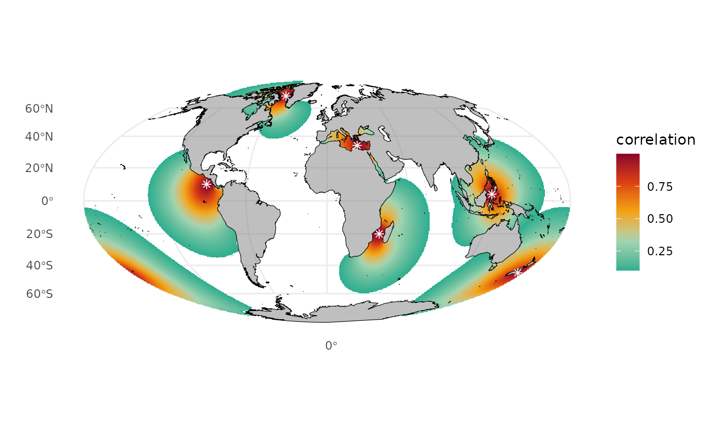
Correlation value for the 2 selected spatial points
Simulation of the space-time barrier model
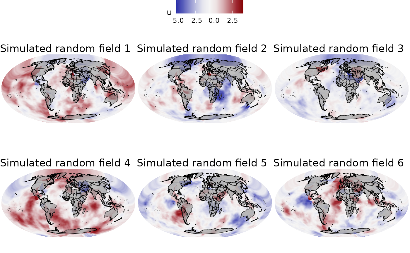
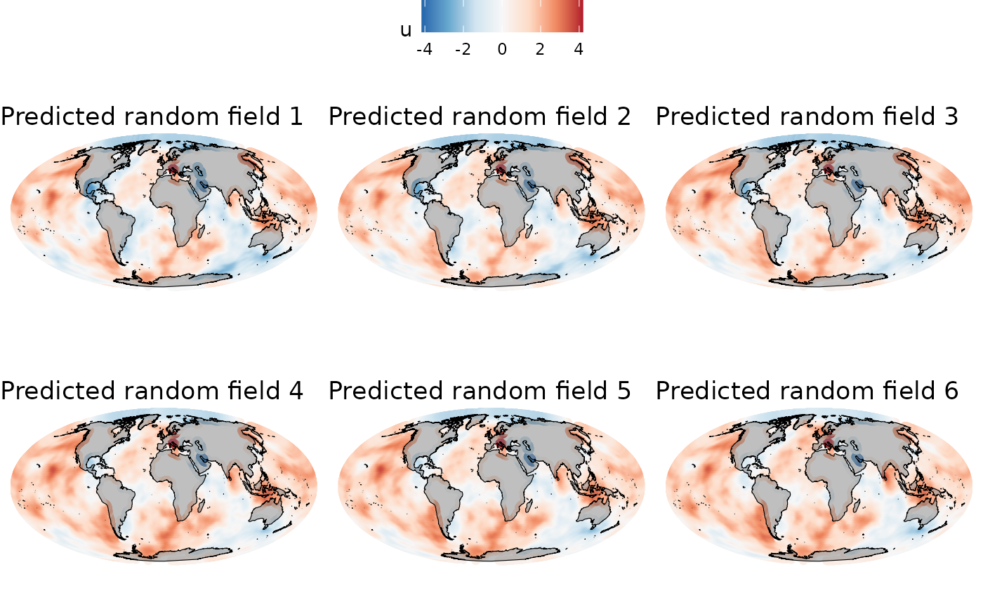
Having established the parameters (range and standard deviation) in the previous section and verified their properties, we can proceed to compute the simulated random field for the barrier model. Subsequently, we can project the random field onto the defined grid for visualization. Since we are working in space and time, we have simulated a total of 6 random fields.
## Number of years k
k <- 6

## Initialize lists to store random seeds and spatial fields
seed <- c(345,1,123,663,2314,654)
u <- list()

## Generate random samples for each spatial field
for(i in 1:k) {
  u[[i]] <- inla.qsample(1, Q, seed = seed[[i]])
}

## Project the field grid onto the Mollweide projection
grid_sf <- list()
for(i in 1:k) {
  grid_sf[[i]] <- st_as_sf(data.frame(
    st_coordinates(mgrid),
    u_proj = inla.mesh.project(gproj, as.vector(u[[i]]))),
    coords = 1:2, crs = crs_vis)
}
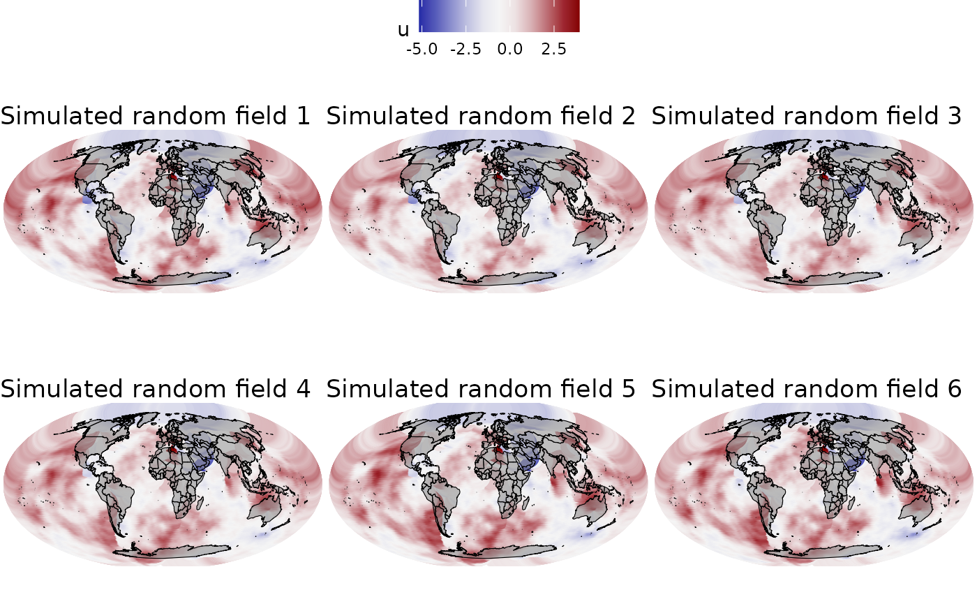
Then, to ensure they are not independent from each other, we are going to correlate them using an autoregressive model of order 1 (AR1).
## Autoregressive smoothing
rho <- 0.98
u_time <- u
for(i in 2:k) {
  u_time[[i]] <- rho * u_time[[i-1]] + sqrt(1-rho^2) * u_time[[i]]
}

## Project the field grid onto the Mollweide projection
grid_sf_u <- list()
for(i in 1:k) {
  grid_sf_u[[i]] <- st_as_sf(data.frame(
    st_coordinates(mgrid),
    u_proj = inla.mesh.project(gproj, as.vector(u_time[[i]]))),
    coords = 1:2, crs = crs_vis)
}Simulation of locations
Regarding the simulation of the response variable, we first need to determine a set of locations where our variable will be observed. To achieve this, we simulate n values from a polygon within the limits of our domain, and the observations will vary for each time. Note that the simulation of locations takes into account a coordinate reference system (CRS). Without a CRS, there would be a disproportionately large number of points near the poles compared to the equator. This discrepancy arises due to the Earth’s shape, and utilizing a CRS helps maintain a more balanced and accurate representation in our simulations.
## Generate random data locations in longlat
## Create world-size sampling area without crs
world_poly_wgs84 <- Earth_poly(resol = 100)

## Add WGS84 crs to a duplicated object
st_crs(world_poly_wgs84) <- 4326

## convert to the Mollweid projection
world_poly_planar <- st_transform(
  x = world_poly_wgs84,
  crs = crs_vis
)

## Sample the locations for each time
set.seed(34521)
## Number of observations
n <- 5000
sf::sf_use_s2(FALSE)
locs_mll <- list()
## Random sampling
seed_2 <- c(34521, 323,43454,24213,2311,2344)
for(i in 1:k) {
  set.seed(seed_2[[i]])
  locs_mll[[i]] <- sf::st_sample(world_poly_planar, n, type = "random",
                                 oriented=TRUE,
                                 exact = TRUE)
}

## Transform data locations to the longlat projection
locs_ll <- list()
for(i in 1:k) {
  locs_ll[[i]] <- st_transform(locs_mll[[i]], crs = st_crs(world_poly_wgs84))
}
Point out that we need to exclude all points that are inside a barrier, as our response variable cannot be observed inside.
## Identify locations outside the world polygon in Mollweide projection
ilocs_in <- list()
locs <- list()
for(i in 1:k) {
  ilocs_in[[i]] <- which(sapply(st_intersects(
    locs_mll[[i]], world_barrier), length) == 0)
  ## extract the coordinates
  locs[[i]] <- st_coordinates(locs_ll[[i]])[ilocs_in[[i]], ]
}
Furthermore, we transform the points onto the sphere using the fm_transform function, allowing us to fit the model later on in 3D.
## Map the data locations back to the sphere
locs_sph <- list()
for(i in 1:k) {
  locs_sph[[i]] <- fm_transform(
    x = locs_mll[[i]][ilocs_in[[i]]],
    crs = fm_crs("sphere"))
}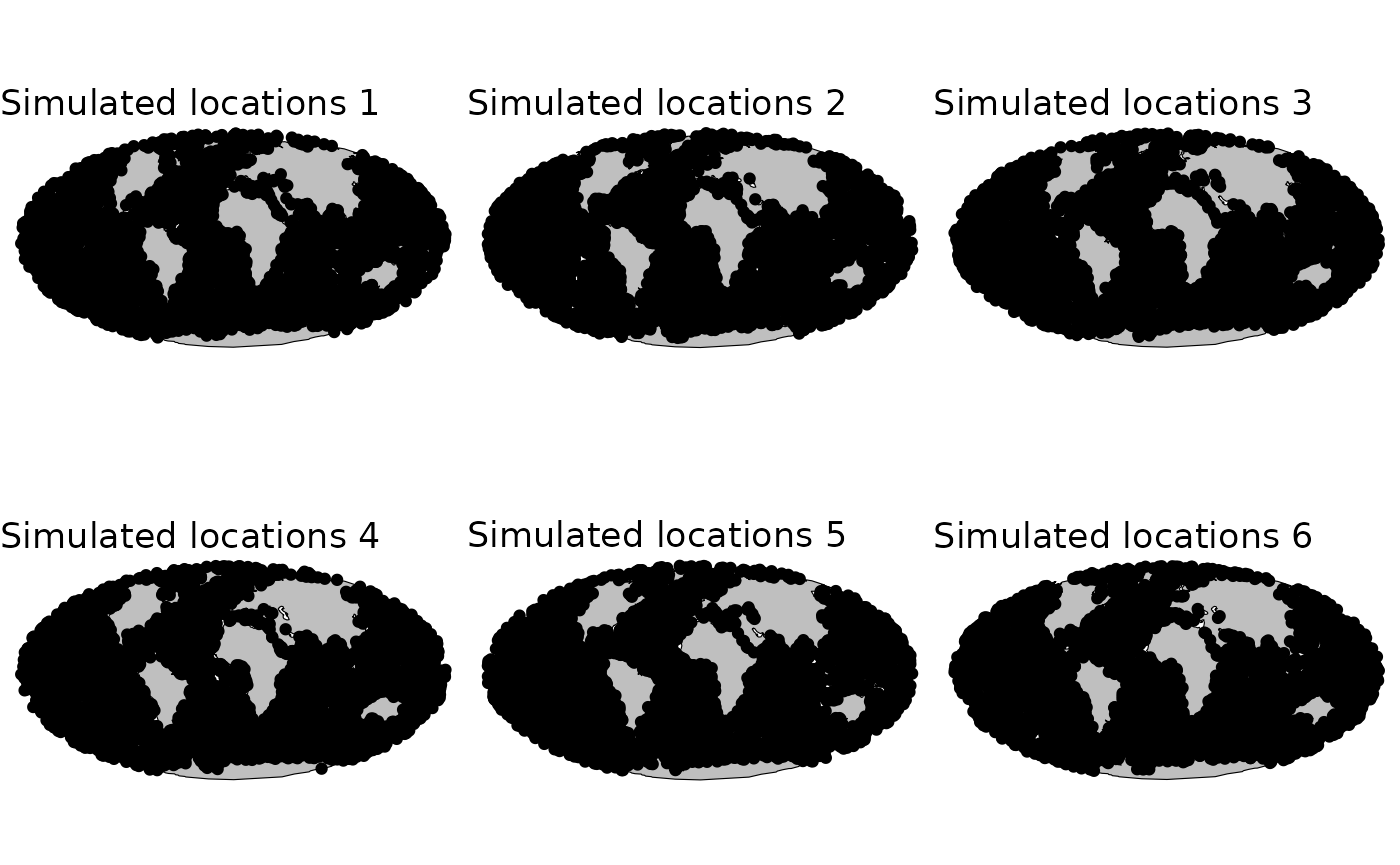
Spatial points where we have observed the response variable
Covariate: depth
Here, we aim to include a continuous covariate with a linear effect. For that, we are going to use the ocean depth and consider a negative linear effect. Note that to download the depth data, you need to run this in R outside of Quarto or Rmarkdown. You only need to do this once.
depth_values <- list()
for(i in 1:k) {
      depth_values[[i]] <- get_depth(as.data.frame(locs[[i]]))
}
We have some missing data, so we are going to eliminate those locations that do not have any depth associated.
## Create a new data frame 'locs_latlong' with columns 'x', 'y', and 'depth'
locs_latlong <- list()
for(i in 1:k) {
 locs_latlong[[i]] <- data.frame(x = depth_values[[i]]$X,
                           y = depth_values[[i]]$Y,
                           depth = depth_values[[i]]$depth)
}

## Use 'depth' in kilometers for easier interpretation in the 'locs_latlong' data frame
for(i in 1:k) {
 locs_latlong[[i]]$depth <- as.vector(locs_latlong[[i]]$depth / 1000)
}

## Remove rows with missing values in the 'locs_latlong' data frame
for(i in 1:k) {
  locs_latlong[[i]] <- na.omit(locs_latlong[[i]])
}

## Calculate the new number of rows in the modified 'locs_latlong' data frame
n_new <- list()
for(i in 1:k) {
  n_new[[i]] <- nrow(locs_latlong[[i]])
}

## Create a spatial features object (sf)
depth_sf <- list()
depth_mll <- list()
for(i in 1:k) {
 depth_sf[[i]] <- st_as_sf(locs_latlong[[i]], coords = c(1, 2), crs = crs_ll)
 depth_mll[[i]] <- st_transform(depth_sf[[i]], crs = crs_vis)
}
Finally, after removing all the missing data, we can update the previously simulated locations to retain only points where we have a corresponding depth value. We have projected the filtered locations onto the sphere using the fm_transform function.
## Transform from data.frame to sf object
locs_filter <- list()
for(i in 1:k) {
  locs_filter[[i]] <- st_as_sf(locs_latlong[[i]],
                               coords = c("x", "y"), crs = crs_ll)
}

## Map the data locations back to the sphere
locs_sph <- list()
for(i in 1:k) {
  locs_sph[[i]] <- fm_transform(
    x = locs_filter[[i]],
    crs = fm_crs("sphere"))
}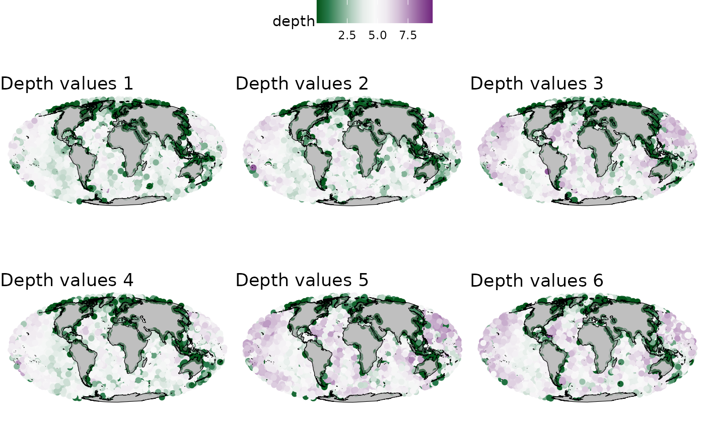
Scale values of depth in the selected locations
Response variable space and space-time
In this tutorial, we will fit four different scenarios: 1) a spatial Normal response variable, 2) a spatial Bernoulli response variable, 3) a space-time Normal response variable, and 4) a space-time Bernoulli response variable. Therefore, we have two spatial scenarios and another two space-time scenarios. Likewise, we will illustrate how to fit Normal and Bernoulli distributions.
Space-time response variables
Next, we are going to simulate the same response variables, but including the time effect. Therefore, we will have two different space-time datasets: one for a Normal response variable and another one with a Bernoulli response variable.
Normal distribution
For the normal response variable, we will use all the simulated random fields. Subsequently, we will prepare a data.frame with the coordinates in the sphere and values of depth and the simulated response at those coordinates for fitting the model.
## Create sparse precision matrices for data locations
Alocs_time <- list()
for(i in 1:k) {
  Alocs_time[[i]] <- inla.spde.make.A(
    mesh = smesh, loc = locs_sph[[i]])
}

## Set parameters for data simulation
beta0_norm <- 10 ## Intercept
beta1_norm <- -1.5 ## Depth coefficient
sigma_e <- 0.3 ## Gaussian standard deviation

## Simulate the response variable y
set.seed(356)
y_norm_t <- list()
for(i in 1:k) {
  y_norm_t[[i]] <- rnorm(n_new[[i]], beta0_norm +
                           beta1_norm * locs_latlong[[i]]$depth +
                           drop(Alocs_time[[i]] %*% u_time[[i]]), sigma_e)
}

## Create a data frame for the simulated data
data_f_norm_t <- list()
for(i in 1:k) {
 data_f_norm_t[[i]] <- st_as_sf(
  data.frame(
    locs_latlong[[i]][,c(1,2)],
    z = y_norm_t[[i]]),
  coords = c(1, 2),
  crs = crs_ll)
}

## Visualize the simulated data on the Mollweide projection
data_mll_norm_t <- list()
locs_mll_data_norm_t <- list()
for(i in 1:k) {
 data_mll_norm_t[[i]] <- st_transform(data_f_norm_t[[i]], crs = crs_vis)
locs_mll_data_norm_t[[i]] <- st_coordinates(data_mll_norm_t[[i]])
}

## Combine data from all time steps for modeling
data_model_norm_t <- data.frame()
for (i in 1:k) {
  coordinates <- locs_sph[[i]]
  y_response <- data_mll_norm_t[[i]]$z
  depth <- locs_latlong[[i]]$depth

  data_model_norm_t <- rbind(data_model_norm_t, data.frame(
    time = rep(i, nrow(st_coordinates(coordinates))),
    y = y_response,
    depth = depth,
    x_coord = st_coordinates(coordinates)[,1],
    y_coord = st_coordinates(coordinates)[,2],
    z_coord = st_coordinates(coordinates)[,3]
  ))
} 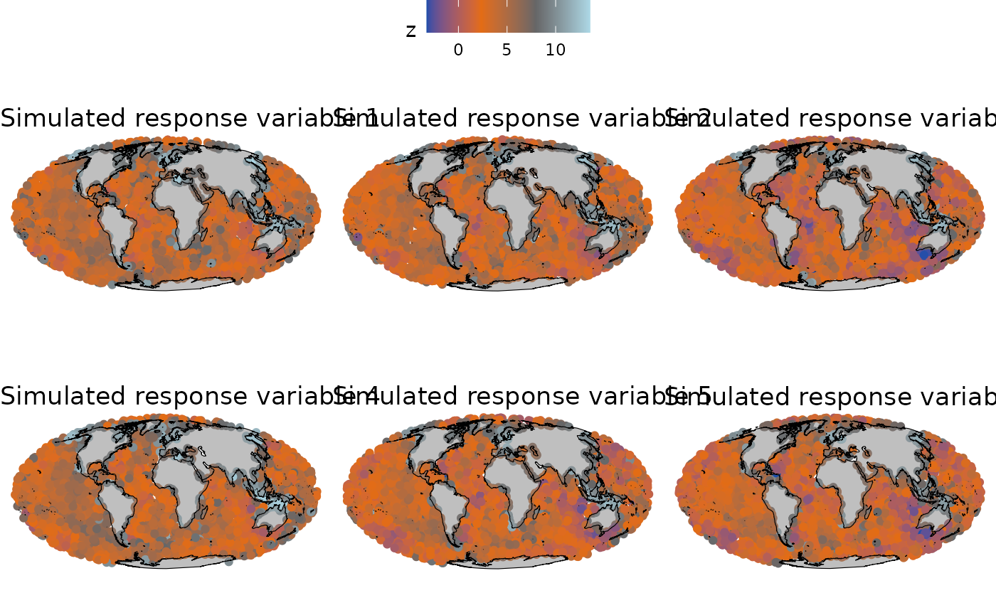
Values of the response variable over the space and time
Bernouilli distribution
Then, for the Bernoulli distribution, we follow the same steps, but considering the probability as the parameter of interest.
## Set parameters for data simulation
beta0_ber <- 1 ## Intercept
beta1_ber <- -1.5 ## Depth coefficient

## Simulated probability
p_time <- list()
for(i in 1:k) {
  p_time[[i]] <- boot::inv.logit(beta0_ber +
                       beta1_ber * locs_latlong[[i]]$depth +
                       drop(Alocs_time[[i]] %*% u_time[[i]]))
}

## Data.frame with the probability
data_prob_t <- list()
for(i in 1:k) {
  data_prob_t[[i]] <- data.frame(locs_latlong[[i]],
                        prob = p_time[[i]])
}

set.seed(356)
y_ber_t <- list()
for(i in 1:k) {
  y_ber_t[[i]] <- rbinom(n = length(data_prob_t[[i]]$prob), 1, prob = data_prob_t[[i]]$prob)
  data_prob_t[[i]]$response <- y_ber_t[[i]]
}


## Create a data frame for the simulated data
data_f_ber_t <- list()
for(i in 1:k) {
  data_f_ber_t[[i]] <- st_as_sf(
  data.frame(
    locs_latlong[[i]][,c(1,2)],
    z = data_prob_t[[i]]$response
  ),
  coords = c(1, 2),
  crs = crs_ll)
}

## Visualize the simulated data on the Mollweide projection
data_mll_ber_t <- list()
locs_mll_ber_t <- list()
for(i in 1:k) {
 data_mll_ber_t[[i]] <- st_transform(data_f_ber_t[[i]], crs = crs_vis)
locs_mll_ber_t[[i]] <- st_coordinates(data_mll_ber_t[[i]])
}

## Combine data from all time steps for modeling
data_model_ber_t <- data.frame()
for (i in 1:k) {
  coordinates <- locs_sph[[i]]
  y_response <- data_mll_ber_t[[i]]$z
  depth <- locs_latlong[[i]]$depth

  data_model_ber_t <- rbind(data_model_ber_t, data.frame(
    time = rep(i, nrow(st_coordinates(coordinates))),
    y = y_response,
    depth = depth,
    x_coord = st_coordinates(coordinates)[,1],
    y_coord = st_coordinates(coordinates)[,2],
    z_coord = st_coordinates(coordinates)[,3]
  ))
}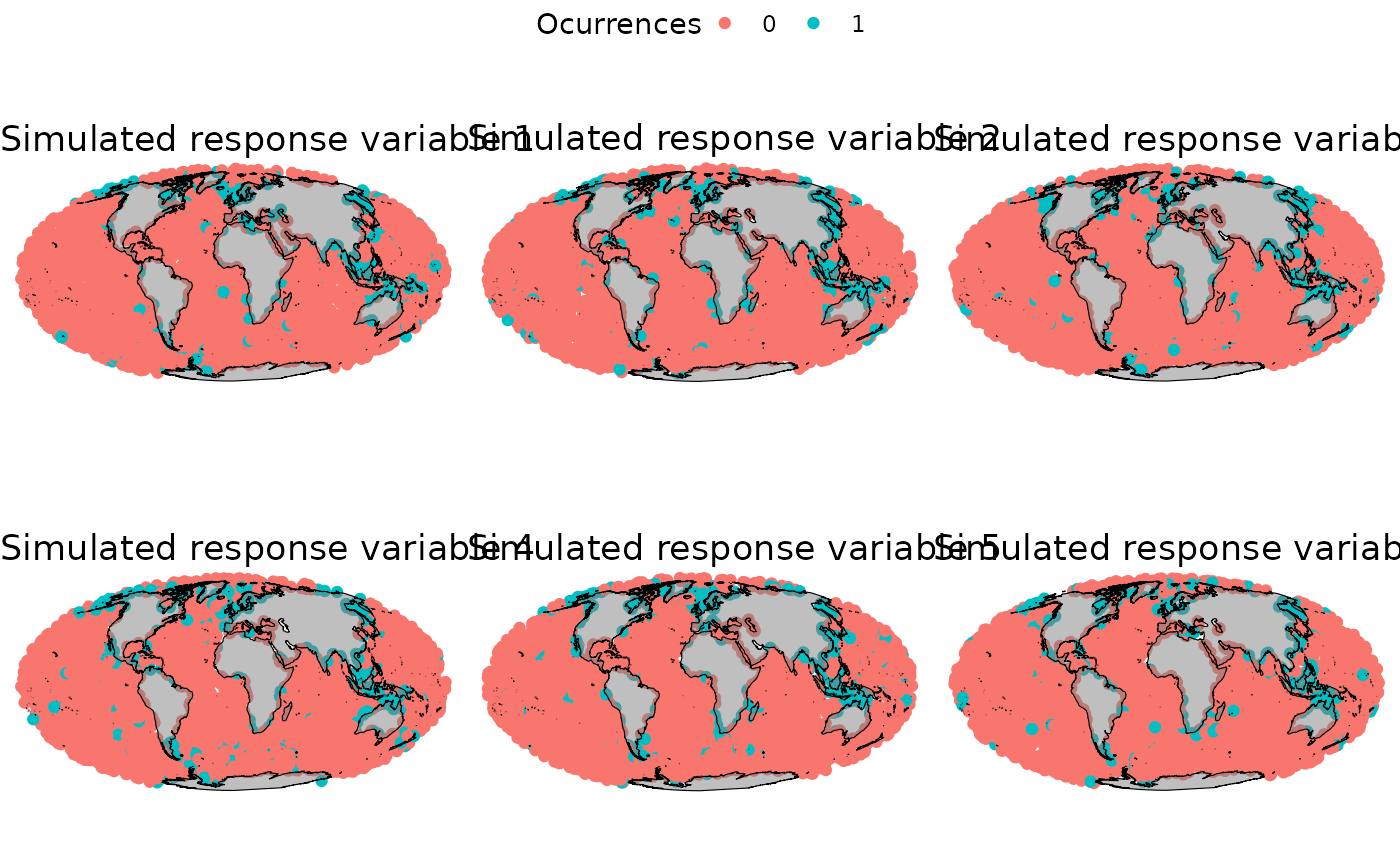
Values of the response variable over the space and time
Fit the barrier model
To begin, we define the model object using the barrierModel.define function. In this step, we specify details such as the mesh, the barrier, the PC priors for the random field hyperparameters, and the fraction of the range when a barrier is in close proximity. This will be the same for all the scenarios.
## Define a barrier model using the mesh and specified prior parameters
bmodel <- barrierModel.define(
  mesh = smesh, ## mesh in 3D
  barrier.triangles = triBarrier, ## Barriers (world countries)
  prior.range = c(0.5, 0.1), ## P(range < 0.5) = 0.1
  prior.sigma = c(1, 0.1), ## P(range > 1) = 0.1
  range.fraction = 0.008 ## range at the barriers
)
We will fit the model using both the inla base code and inlabru. For both approaches, it is necessary to create a data.frame containing the three-dimensional location, depth values, and the simulated response variable values.
Spatial scenarios
Normal response variable
INLABRU
We use the model formula in the inlabru way, where field will be the name of the spatial effect. The main function in inlabru is bru, and we just need to specify the model formula (model), the data (dataset), and the family (gaussian). We also turn on the verbose argument to be able to see the fitting process while it is running.
## Specify the model formula
model_norm <- y ~
  ## Intercept
  Intercept(1) +
  ## Depth linear effect
  bat(depth, model = "linear") +
  ## Spatial effect
  field(cbind(x_coord,y_coord,z_coord),
        model = bmodel #The barrier model
        )

## Fit the Bayesian model using INLA
set.seed(2353)
result_norm <- bru(
    model_norm, data_model_norm_t[data_model_norm_t$time == 1,][,-1],
    family = "gaussian",
    options = list(
        verbose = TRUE,
        control.compute = list(cpo = TRUE)))
Once we have fitted the model, we can observe if we get back the results. First, we check the summary of the fixed effect and the hyperparameters.
## Beta 0 (intercept) and Beta 1 (depth)
res_summary_fixed_rounded <- round(result_norm$summary.fixed, 2)| mean | sd | 0.025quant | 0.5quant | 0.975quant | mode | kld | |
|---|---|---|---|---|---|---|---|
| Intercept | 10.08 | 0.18 | 9.72 | 10.08 | 10.43 | 10.08 | 0 |
| bat | -1.50 | 0.01 | -1.51 | -1.50 | -1.48 | -1.50 | 0 |
## Range, standard deviation (spatial effect), and standard deviation (Gaussian)
res_summary_hyper_rounded <- round(result_norm$summary.hyperpar, 2)| mean | sd | 0.025quant | 0.5quant | 0.975quant | mode | |
|---|---|---|---|---|---|---|
| Precision for the Gaussian observations | 10.85 | 0.36 | 10.16 | 10.84 | 11.57 | 10.83 |
| Theta1 for field | -0.41 | 0.08 | -0.57 | -0.41 | -0.24 | -0.41 |
| Theta2 for field | 0.05 | 0.07 | -0.09 | 0.05 | 0.19 | 0.04 |
Then, we compute the marginals of the hyperparameters: range , standard deviation of the spatial effect , and standard deviation of the Gaussian distribution .
## Create a list of hyperparameter marginals for visualization
pmarginals <-
  list(
    data.frame(
      param = "sigma.e",
      inla.tmarginal(
        function(x) exp(-x/2),
        result_norm$internal.marginals.hyperpar$`Log precision for the Gaussian observations`)),
    data.frame(
      param = "range",
      inla.tmarginal(
        function(x) exp(x),
        result_norm$internal.marginals.hyperpar$`Theta1 for field`)),
    data.frame(
      param = "sigma",
      inla.tmarginal(
        function(x) exp(x),
        result_norm$internal.marginals.hyperpar$`Theta2 for field`))
  )

## Add true values and quantiles to hyperparameter marginals
pmarginals[[1]]$true <- rep(sigma_e, length(pmarginals[[1]]$x))
pmarginals[[2]]$true <- rep(ranges[1], length(pmarginals[[1]]$x))
pmarginals[[3]]$true <- rep(1, length(pmarginals[[1]]$x))
Likewise, we can plot the marginals for the fixed effects: intercept and depth linear coefficients.
## Create a list of parameter marginals for visualization
fmarginals <-
  list(
    data.frame(
      param = "intercept",
      value = result_norm$marginals.fixed$Intercept
    ),
    data.frame(
      param = "depth",
      value = result_norm$marginals.fixed$bat
    )
  )

## Add true values and quantiles to parameter marginals
fmarginals[[1]]$true <- rep(beta0_norm, length(fmarginals[[1]]$value.x))
fmarginals[[2]]$true <- rep(beta1_norm, length(fmarginals[[2]]$value.y))
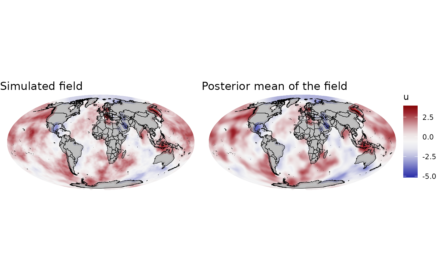
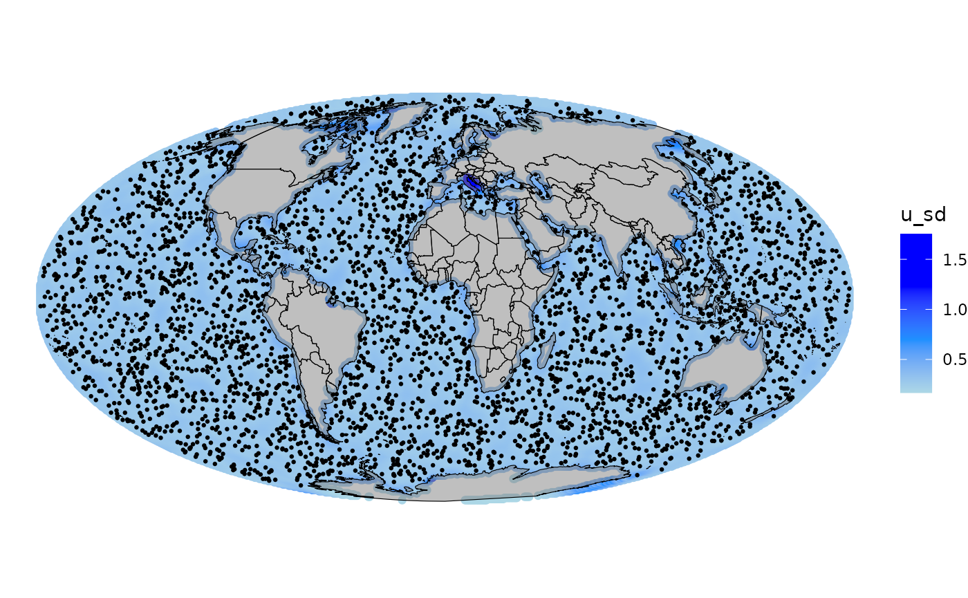
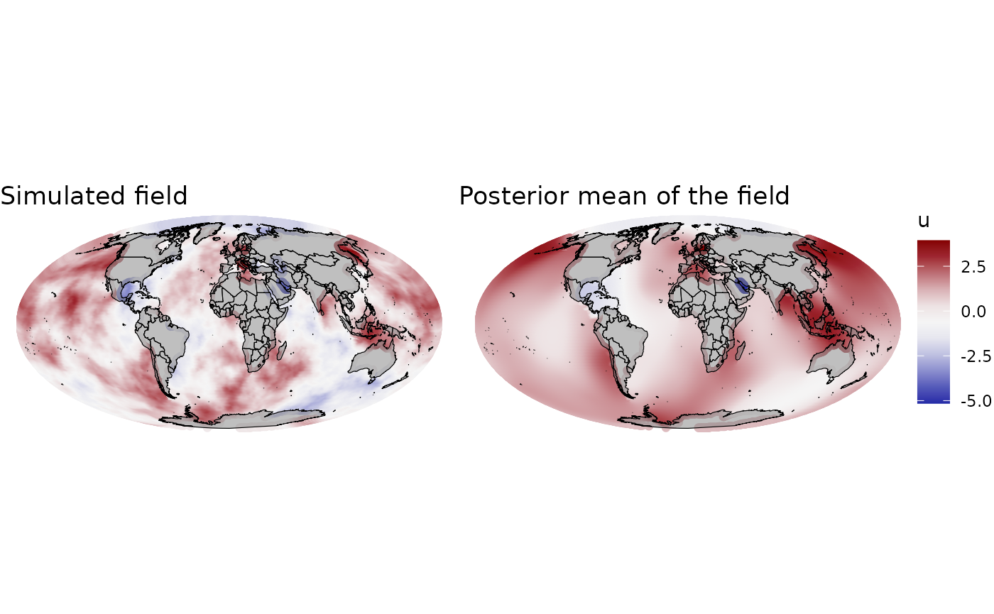
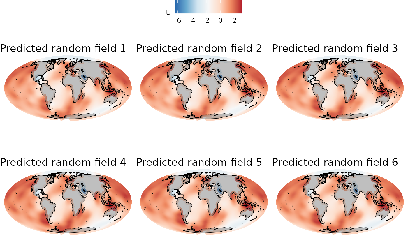
We can also visualize the predicted random field. In this case, we compute the mean of the spatial field and also the standard deviation.
## Add mean and standard deviation of the field to the grid
grid_sf[[1]]$u_mean <- as.vector( ## mean
  inla.mesh.project(
      gproj,
      result_norm$summary.random$field$mean))

grid_sf[[1]]$u_sd <- exp(as.vector( ## standard deviation
  inla.mesh.project(
    gproj,
    log(result_norm$summary.random$field$sd))))
Hyperparameters posterior distributions
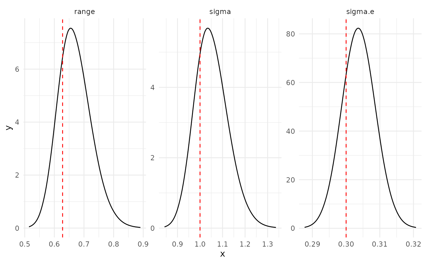
Marginals posterior distributions for the hyperparameters (red line represents the true value)
Fixed parameters
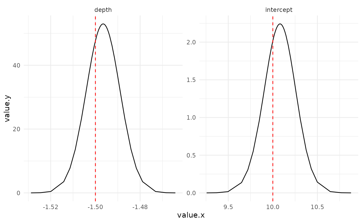
Marginals posterior distributions for the fixed parameters (red line represents the true value)
INLA
The following code fits the model using the INLA base code. To accomplish this, an INLA stack is initially created to model a response variable according to a specified formula. This stack includes a projector matrix (Alocs), spatial effect (i), depth (beta1), and an intercept (beta0).
## Create an INLA stack (stk) for modeling the response variable based on the specified formula and data
stk <- inla.stack(
  data = list(resp = data_model_norm_t[data_model_norm_t$time == 1,]$y), ## Response variable
  A = list(Alocs_time[[1]], 1,1),  ## Projector matrix
  effects = list(i = 1:bmodel$mesh$n, ## Spatial effect
                 beta1 = data_model_norm_t[data_model_norm_t$time == 1,]$depth, ## Depth
                 beta0 = rep(1,nrow(data_model_norm_t[data_model_norm_t$time == 1,])) ## Intercept
  ),
  tag = "est" ## Estimation stack (est)
)

## Use inla to fit the specified formula and obtain the result
set.seed(52134)
result_norm <- inla(resp ~ 0 + beta0 + f(beta1, model = "linear") + f(i, model = bmodel), ## Formula
            data = inla.stack.data(stk), ## Stack
            control.predictor = list(A = inla.stack.A(stk),
                                     compute = TRUE),
            control.compute = list(return.marginals.predictor = TRUE),
            verbose = TRUE)
Once we have fitted the model, we can observe if we get back the results. First, we check the summary of the fixed effect and the hyperparameters.
## Beta 0 (intercept) and Beta 1 (depth)
res_summary_fixed_rounded <- round(result_norm$summary.fixed, 2)| mean | sd | 0.025quant | 0.5quant | 0.975quant | mode | kld | |
|---|---|---|---|---|---|---|---|
| beta0 | 10.08 | 0.18 | 9.72 | 10.08 | 10.43 | 10.08 | 0 |
| beta1 | -1.50 | 0.01 | -1.51 | -1.50 | -1.48 | -1.50 | 0 |
## Range, standard deviation (spatial effect), and standard deviation (Gaussian)
res_summary_hyper_rounded <- round(result_norm$summary.hyperpar, 2)| mean | sd | 0.025quant | 0.5quant | 0.975quant | mode | |
|---|---|---|---|---|---|---|
| Precision for the Gaussian observations | 10.85 | 0.36 | 10.16 | 10.84 | 11.57 | 10.83 |
| Theta1 for i | -0.41 | 0.08 | -0.56 | -0.41 | -0.24 | -0.41 |
| Theta2 for i | 0.05 | 0.07 | -0.09 | 0.05 | 0.19 | 0.04 |
Then, we compute the marginals of the hyperparameters: ranges , standard deviation of the spatial effect , and standard deviation of the Gaussian distribution .
## Create a list of parameter marginals for visualization
pmarginals <-
  list(
    data.frame(
      param = "sigma.e",
      inla.tmarginal(
        function(x) exp(-x/2),
        result_norm$internal.marginals.hyperpar$`Log precision for the Gaussian observations`)),
    data.frame(
      param = "range",
      inla.tmarginal(
        function(x) exp(x),
        result_norm$internal.marginals.hyperpar$`Theta1 for i`)),
    data.frame(
      param = "sigma",
      inla.tmarginal(
        function(x) exp(x),
        result_norm$internal.marginals.hyperpar$`Theta2 for i`))
  )

## Add true values to parameter marginals
pmarginals[[1]]$true <- rep(sigma_e, length(pmarginals[[1]]$x))
pmarginals[[2]]$true <- rep(ranges[1], length(pmarginals[[1]]$x))
pmarginals[[3]]$true <- rep(1, length(pmarginals[[1]]$x))
Likewise, we can plot the marginals for the fixed parameters: intercept and depth linear coefficient.
## Create a list of parameter marginals for visualization
fmarginals <-
  list(
    data.frame(
      param = "intercept",
      value = result_norm$marginals.fixed$beta0
    ),
    data.frame(
      param = "depth",
      value = result_norm$marginals.fixed$beta1
    )
  )

## Add true values to parameter marginals
fmarginals[[1]]$true <- rep(beta0_norm, length(fmarginals[[1]]$value.x))
fmarginals[[2]]$true <- rep(beta1_norm, length(fmarginals[[2]]$value.y))
We can also visualize the predicted random field. In this case, we compute the mean of the spatial field and also the standard deviation.
## Add mean and standard deviation of the field to the grid
grid_sf[[1]]$u_mean <- as.vector( ## mean
  inla.mesh.project(
      gproj,
      result_norm$summary.random$i$mean))

grid_sf[[1]]$u_sd <- exp(as.vector( ## standard deviation
  inla.mesh.project(
    gproj,
    log(result_norm$summary.random$i$sd))))
Hyperparameters posterior distributions

Marginals posterior distributions for the hyperparameters (red line represents the true value)
Fixed parameters
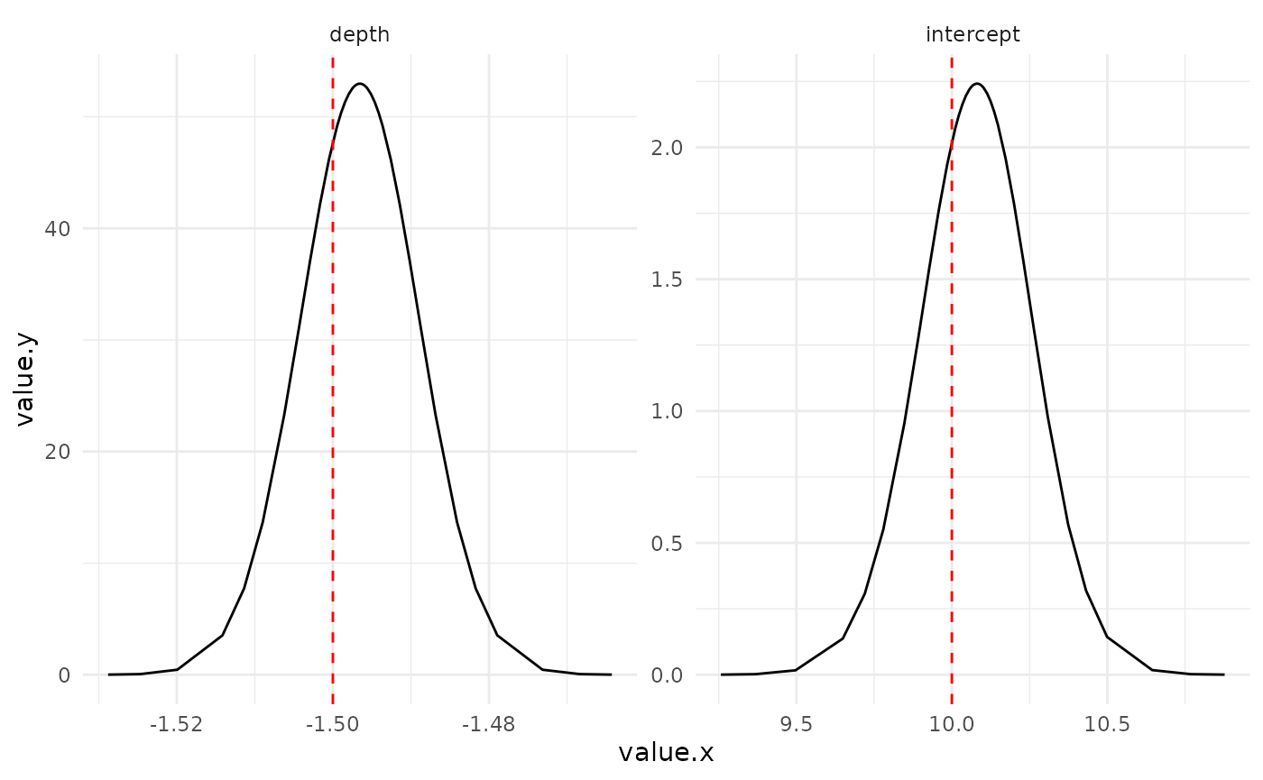
Marginals posterior distributions for the fixed parameters (red line represents the true value)
Prediction
Another common objective with these models is to predict the response variable in unsampled locations. Here, we share the code for predicting with the barrier model across the Earth. Initially, we must download the depth values for the locations we want to predict. In this case, we’ll utilize the grid previously defined for projecting the random field.
## Extracting latitude and longitude from the defined grid
locs_latlong_pred <- get_depth(data = as.data.frame(
st_coordinates(grid_ll[[1]])))

## Scale the depth values (to km units) and storing them in the 'depth' column
locs_latlong_pred$depth <- as.vector(locs_latlong_pred$depth / 1000)
Next, we have to set up the stack for prediction. Here, the response variable is defined with NA (not available), and we replicate the same effects present in the stack for estimation but with the updated depth values. Lastly, we merge both stacks, combining those for estimation and prediction.
## Create an inla.stack object for prediction
stk.pred <- inla.stack(
  data = list(resp = NA), ## Placeholder for the response variable (to be predicted)
  A = list(gproj$proj$A, 1, 1), ## Projection matrix for the spatial field and an intercept term
  effects = list(i = 1:bmodel$mesh$n, ## Spatial random effect
                 beta1 = locs_latlong_pred$depth,
                 beta0 = rep(1, length(locs_latlong_pred$depth))), ## Intercept term
  tag = "pred" ## Tag for the stack, indicating it is used for prediction
)

## Combine the original stack (stk) with the prediction stack (stk.pred)
stk.full <- inla.stack(stk, stk.pred)
Once we have our complete stack, we can rerun the model exclusively for prediction, utilizing the previously fitted results (adjust this in control.mode).
## Re-run the model
set.seed(52134)
res_pred <- inla(resp ~ 0 + beta0 + f(beta1, model = "linear") + f(i, model = bmodel), ## Formula
                 data = inla.stack.data(stk.full), ## Stack
                 control.mode = list(theta = result_norm$mode$theta, restart = FALSE), ##  Utilize the theta parameters obtained from the previously estimated spde model
                 control.predictor = list(A = inla.stack.A(stk.full),
                                          compute = TRUE),
                 control.compute = list(return.marginals.predictor = TRUE),
                 verbose = TRUE)
In the end, we extract the predicted values from the model and generate an sf object for visualization.
## Extracting the values of the response variable
pred <- inla.stack.index(stk.full, "pred")$data
pred_values <- res_pred$summary.fitted.values$mean[pred]

## Creating a data frame with coordinates and predicted values
data_raster_pred <- data.frame(x = st_coordinates(grid_ll)[,1],
                               y = st_coordinates(grid_ll)[,2],
                               pred = as.vector(pred_values)
)

## Creating an sf object for visualization in Mollweide projection
data_pred <- st_as_sf(x = data_raster_pred,
                      coords = c("x","y"),
                      crs = crs_ll)

## Transforming the sf object to the desired projection
data_pred_mll <- st_transform(data_pred, crs = crs_vis)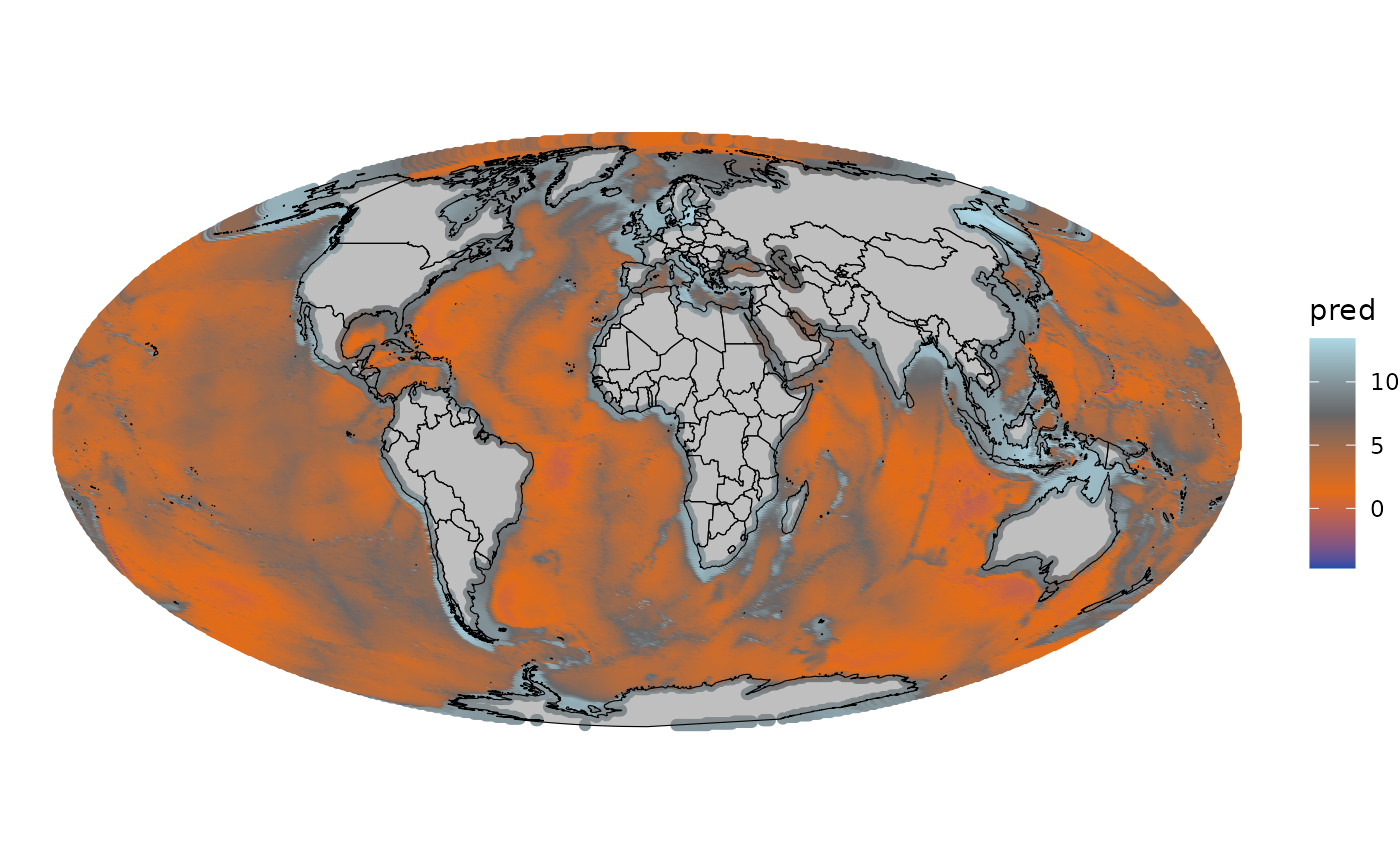
Predicted response variable across the entire domain
Bernouilli response variable
We will use the same code provided for the normal response variable to fit the Bernoulli distribution, with slight modifications to specify the likelihood.
INLABRU
First, we will establish the components of the model and indicate that our response variable follows a Bernoulli distribution.
## Specify the model formula
model_ber <- y ~
  ## Intercept
  Intercept(1) +
  ## Depth linear effect
  bat(depth, model = "linear") +
  ## Spatial effect
  field(cbind(x_coord,y_coord,z_coord),
        model = bmodel #The barrier model
        )

## Fit the Bayesian model using INLA
set.seed(2353)
result_ber <- bru(
    model_ber, data_model_ber_t[data_model_ber_t$time == 1,][,-1],
    family = "binomial",
    options = list(
        verbose = TRUE,
        control.compute = list(cpo = TRUE)))
Once we have fitted the model, we can observe if we get back the results. First, we check the summary of the fixed effect and the hyperparameters.
## Beta 0 (intercept) and Beta 1 (depth)
res_summary_fixed_rounded <- round(result_ber$summary.fixed, 2)| mean | sd | 0.025quant | 0.5quant | 0.975quant | mode | kld | |
|---|---|---|---|---|---|---|---|
| Intercept | 0.82 | 0.44 | -0.05 | 0.82 | 1.73 | 0.82 | 0 |
| bat | -1.34 | 0.07 | -1.48 | -1.34 | -1.20 | -1.34 | 0 |
## Range, standard deviation (spatial effect), and standard deviation (Gaussian)
res_summary_hyper_rounded <- round(result_ber$summary.hyperpar, 2)| mean | sd | 0.025quant | 0.5quant | 0.975quant | mode | |
|---|---|---|---|---|---|---|
| Theta1 for field | 0.12 | 0.25 | -0.36 | 0.11 | 0.63 | 0.09 |
| Theta2 for field | -0.08 | 0.16 | -0.39 | -0.08 | 0.22 | -0.08 |
Then, we compute the marginals of the hyperparameters: ranges and standard deviation of the spatial effect .
## Create a list of parameter marginals for visualization
pmarginals <-
  list(
    data.frame(
      param = "range",
      inla.tmarginal(
        function(x) exp(x),
        result_ber$internal.marginals.hyperpar$`Theta1 for field`)),
    data.frame(
      param = "sigma",
      inla.tmarginal(
        function(x) exp(x),
        result_ber$internal.marginals.hyperpar$`Theta2 for field`))
  )

## Add true values to parameter marginals
pmarginals[[1]]$true <- rep(ranges[1], length(pmarginals[[1]]$x))
pmarginals[[2]]$true <- rep(1, length(pmarginals[[1]]$x))
Likewise, we can plot the marginals for the fixed effects: intercept and depth linear coefficients.
## Create a list of parameter marginals for visualization
fmarginals <-
  list(
    data.frame(
      param = "intercept",
      value = result_ber$marginals.fixed$Intercept
    ),
    data.frame(
      param = "depth",
      value = result_ber$marginals.fixed$bat
    )
  )

## Add true values to parameter marginals
fmarginals[[1]]$true <- rep(beta0_ber, length(fmarginals[[1]]$value.x))
fmarginals[[2]]$true <- rep(beta1_ber, length(fmarginals[[2]]$value.y))
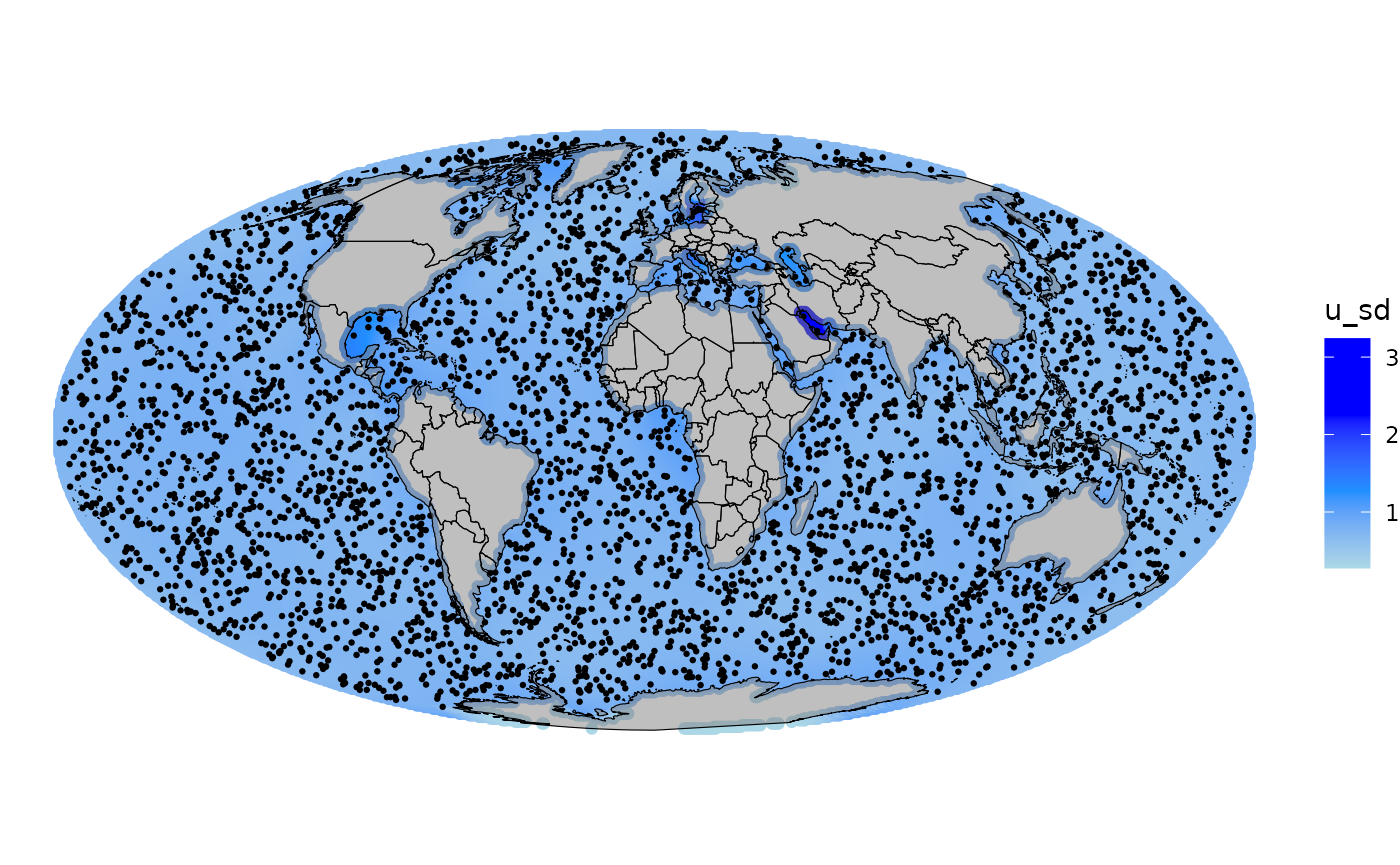
We can also visualize the predicted random field. In this case, we compute the mean of the spatial field and also the standard deviation.
## Add mean and standard deviation of the field to the grid
grid_sf[[1]]$u_mean <- as.vector( ## mean
  inla.mesh.project(
      gproj,
      result_ber$summary.random$field$mean))

grid_sf[[1]]$u_sd <- exp(as.vector( ## standard deviation
  inla.mesh.project(
    gproj,
    log(result_ber$summary.random$field$sd))))
Hyperparameters posterior distributions
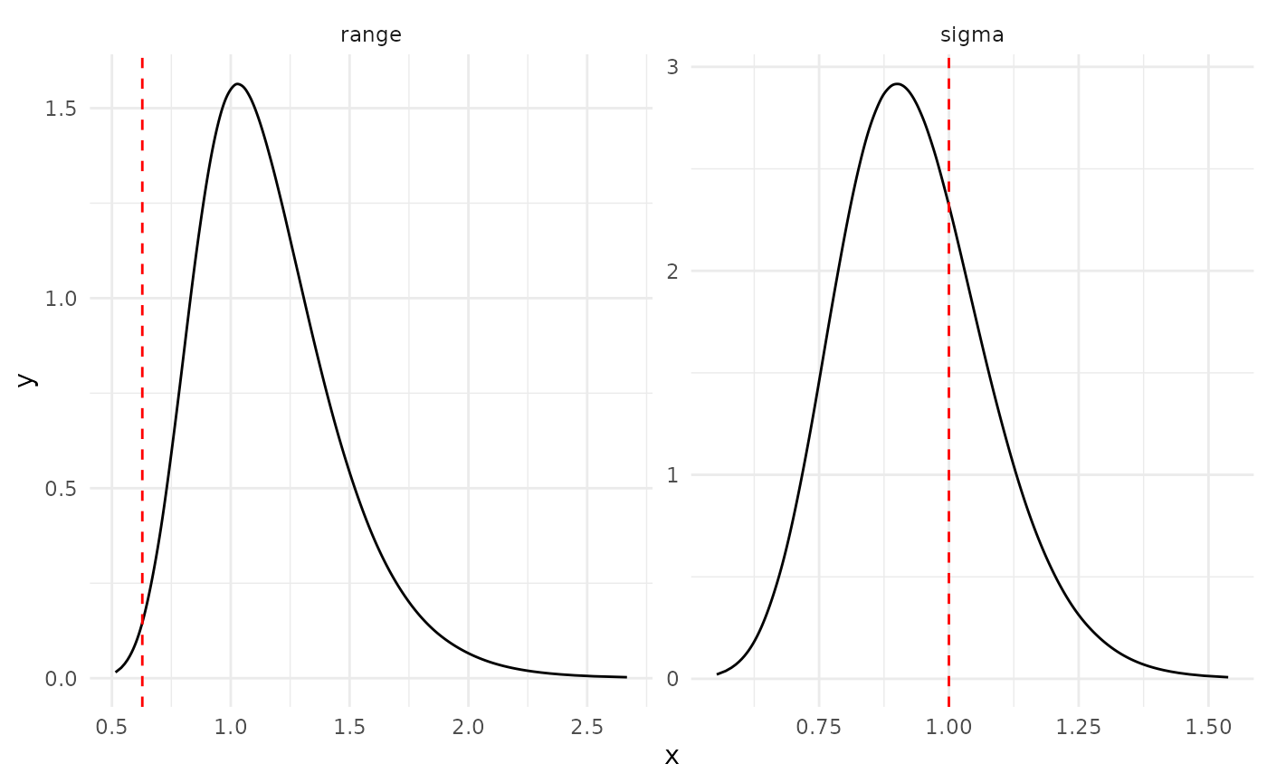
Marginals posterior distributions for the hyperparameters (red line represents the true value)
Fixed parameters
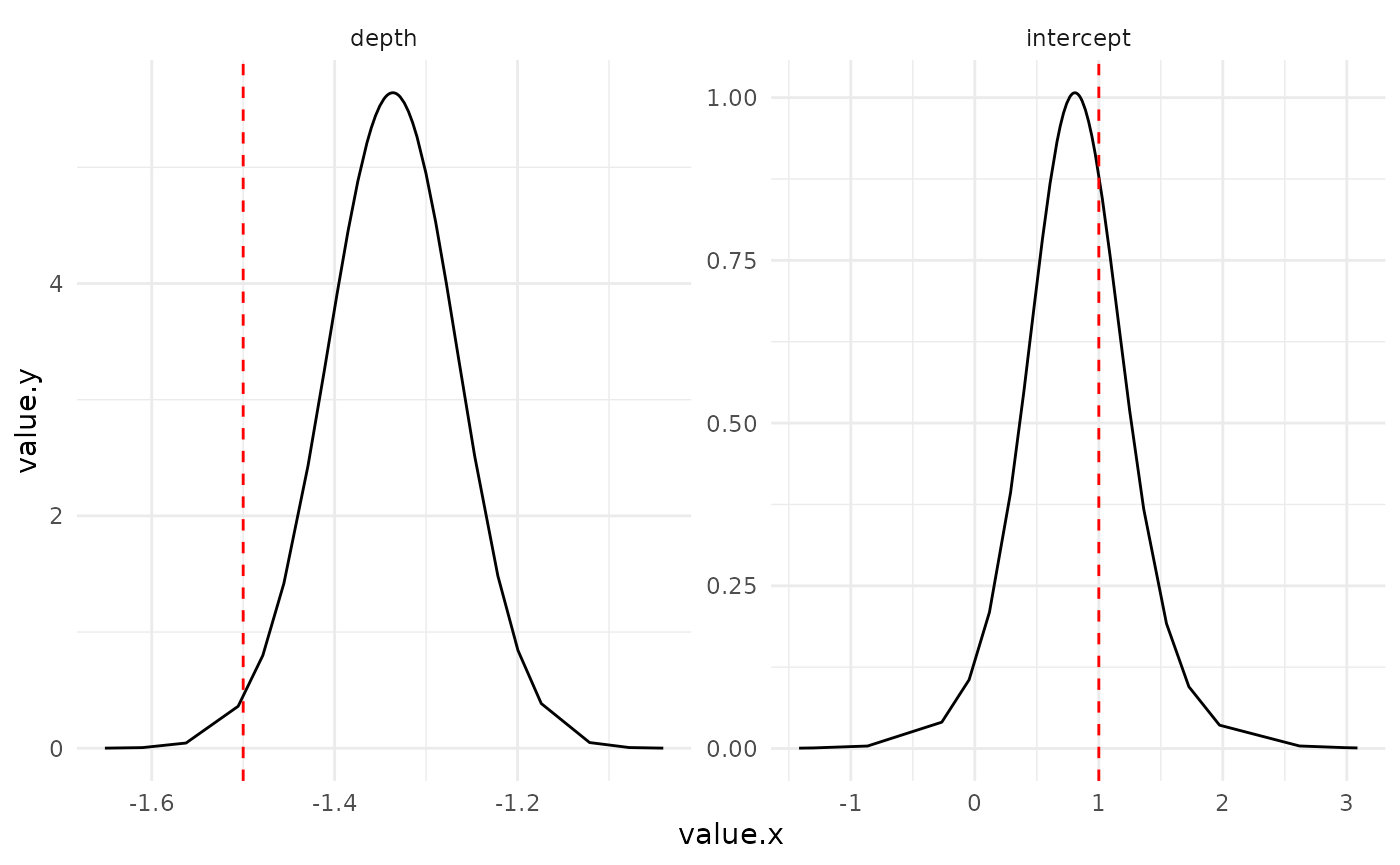
Marginals posterior distributions for the fixed parameters (red line represents the true value)
INLA
The following code fits the model using the INLA base code. To accomplish this, an INLA stack is initially created to model a response variable according to a specified formula. This stack includes a projector matrix (Alocs), spatial effect (i), depth (beta1), and an intercept (beta0).
## Create an INLA stack (stk) for modeling the response variable based on the specified formula and data
stk <- inla.stack(
  data = list(resp = data_model_ber_t[data_model_ber_t$time == 1,]$y), ## Response variable
  A = list(Alocs_time[[1]], 1,1),  ## Projector matrix
  effects = list(i = 1:bmodel$mesh$n, ## Spatial effect
                 beta1 = data_model_ber_t[data_model_ber_t$time == 1,]$depth, ## Depth
                 beta0 = rep(1,nrow(data_model_ber_t[data_model_ber_t$time == 1,])) ## Intercept
  ),
  tag = "est" ## Estimation stack (est)
)

## Use inla to fit the specified formula and obtain the result
set.seed(52134)
result_ber <- inla(resp ~ 0 + beta0 + f(beta1, model = "linear") + f(i, model = bmodel), ## Formula
               data = inla.stack.data(stk), ## Stack
               family = 'binomial',
               control.predictor = list(A = inla.stack.A(stk),
                                        compute = TRUE),
               control.compute = list(return.marginals.predictor = TRUE),
               verbose = TRUE)
Once we have fitted the model, we can observe if we get back the results. First, we check the summary of the fixed effect and the hyperparameters.
## Beta 0 (intercept) and Beta 1 (depth)
res_summary_fixed_rounded <- round(result_ber$summary.fixed, 2)| mean | sd | 0.025quant | 0.5quant | 0.975quant | mode | kld | |
|---|---|---|---|---|---|---|---|
| beta0 | 0.82 | 0.44 | -0.05 | 0.82 | 1.73 | 0.82 | 0 |
| beta1 | -1.34 | 0.07 | -1.48 | -1.34 | -1.20 | -1.34 | 0 |
## Range, standard deviation (spatial effect), and standard deviation (Gaussian)
res_summary_hyper_rounded <- round(result_ber$summary.hyperpar, 2)| mean | sd | 0.025quant | 0.5quant | 0.975quant | mode | |
|---|---|---|---|---|---|---|
| Theta1 for i | 0.12 | 0.25 | -0.36 | 0.11 | 0.63 | 0.09 |
| Theta2 for i | -0.08 | 0.16 | -0.39 | -0.08 | 0.22 | -0.08 |
Then, we compute the marginals of the hyperparameters: ranges and standard deviation of the spatial effect .
## Create a list of parameter marginals for visualization
pmarginals <-
  list(
    data.frame(
      param = "range",
      inla.tmarginal(
        function(x) exp(x),
        result_ber$internal.marginals.hyperpar$`Theta1 for i`)),
    data.frame(
      param = "sigma",
      inla.tmarginal(
        function(x) exp(x),
        result_ber$internal.marginals.hyperpar$`Theta2 for i`))
  )

## Add true values to parameter marginals
pmarginals[[1]]$true <- rep(ranges[1], length(pmarginals[[1]]$x))
pmarginals[[2]]$true <- rep(1, length(pmarginals[[1]]$x))
Likewise, we can plot the marginals for the fixed effects: intercept and depth linear coefficients.
## Create a list of parameter marginals for visualization
fmarginals <-
  list(
    data.frame(
      param = "intercept",
      value = result_ber$marginals.fixed$beta0
    ),
    data.frame(
      param = "depth",
      value = result_ber$marginals.fixed$beta1
    )
  )

## Add true values to parameter marginals
fmarginals[[1]]$true <- rep(beta0_ber, length(fmarginals[[1]]$value.x))
fmarginals[[2]]$true <- rep(beta1_ber, length(fmarginals[[2]]$value.y))
We can also visualize the predicted random field. In this case, we compute the mean of the spatial field and also the standard deviation.
## Add mean and standard deviation of the field to the grid
grid_sf[[1]]$u_mean <- as.vector( ## mean
  inla.mesh.project(
      gproj,
      result_ber$summary.random$i$mean))

grid_sf[[1]]$u_sd <- exp(as.vector( ## standard deviation
  inla.mesh.project(
    gproj,
    log(result_ber$summary.random$i$sd))))
Hyperparameters posterior distributions

Marginals posterior distributions for the hyperparameters (red line represents the true value)
Fixed parameters

Marginals posterior distributions for the fixed parameters (red line represents the true value)
Prediction
Now, we will predict the probability of presence according to the fitted model.
## Extracting latitude and longitude from the defined grid
locs_latlong_pred <- get_depth(data = as.data.frame(    st_coordinates(grid_ll[[1]])))

## Scale the depth values (km units) and storing them in the 'depth' column
locs_latlong_pred$depth <- as.vector(locs_latlong_pred$depth / 1000)
Next, we have to set up the stack for prediction. Here, the respons variable is defined with NA (not available), and we replicate the same effects present in the stack for estimation but with the updated depth values. Lastly, we merge both stacks, combining those for estimation and prediction.
## Create an inla.stack object for prediction
stk.pred <- inla.stack(
  data = list(resp = NA), ## Placeholder for the response variable (to be predicted)
  A = list(gproj$proj$A, 1, 1), ## Projection matrix for the spatial field and an intercept term
  effects = list(i = 1:bmodel$mesh$n, ## Spatial random effect
                 beta1 = locs_latlong_pred$depth,
                 beta0 = rep(1, length(locs_latlong_pred$depth))), ## Intercept term
  tag = "pred" ## Tag for the stack, indicating it is used for prediction
)

## Combine the original stack (stk) with the prediction stack (stk.pred)
stk.full <- inla.stack(stk, stk.pred)
Once we have our complete stack, we can rerun the model exclusively for prediction, utilizing the previously fitted results (adjust this in control.mode).
## Re-run the model
set.seed(52134)
res_pred <- inla(resp ~ 0 + beta0 + f(beta1, model = "linear") + f(i, model = bmodel), ## Formula
                 data = inla.stack.data(stk.full), ## Stack
                 family = 'binomial',
                 control.mode = list(theta = result_ber$mode$theta, restart = FALSE), ##  Utilize the theta parameters obtained from the previously estimated spde model
                 control.predictor = list(A = inla.stack.A(stk.full),
                                          compute = TRUE),
                 control.compute = list(return.marginals.predictor = TRUE),
                 verbose = TRUE)
In the end, we extract the predicted values from the model and generate an sf object for visualization.
## Extracting the values of the response variable
pred <- inla.stack.index(stk.full, "pred")$data
pred_values <- res_pred$summary.fitted.values$mean[pred]
pred_values_presences <- boot::inv.logit(pred_values)

## Creating a data frame with coordinates and predicted values
data_raster_pred <- data.frame(x = st_coordinates(grid_ll)[,1],
                               y = st_coordinates(grid_ll)[,2],
                               pred = as.vector(pred_values_presences)
)

## Creating an sf object for visualization in Mollweide projection
data_pred <- st_as_sf(x = data_raster_pred,
                      coords = c("x","y"),
                      crs = crs_ll)

## Transforming the sf object to the desired projection
data_pred_m <- st_transform(data_pred, crs = crs_vis)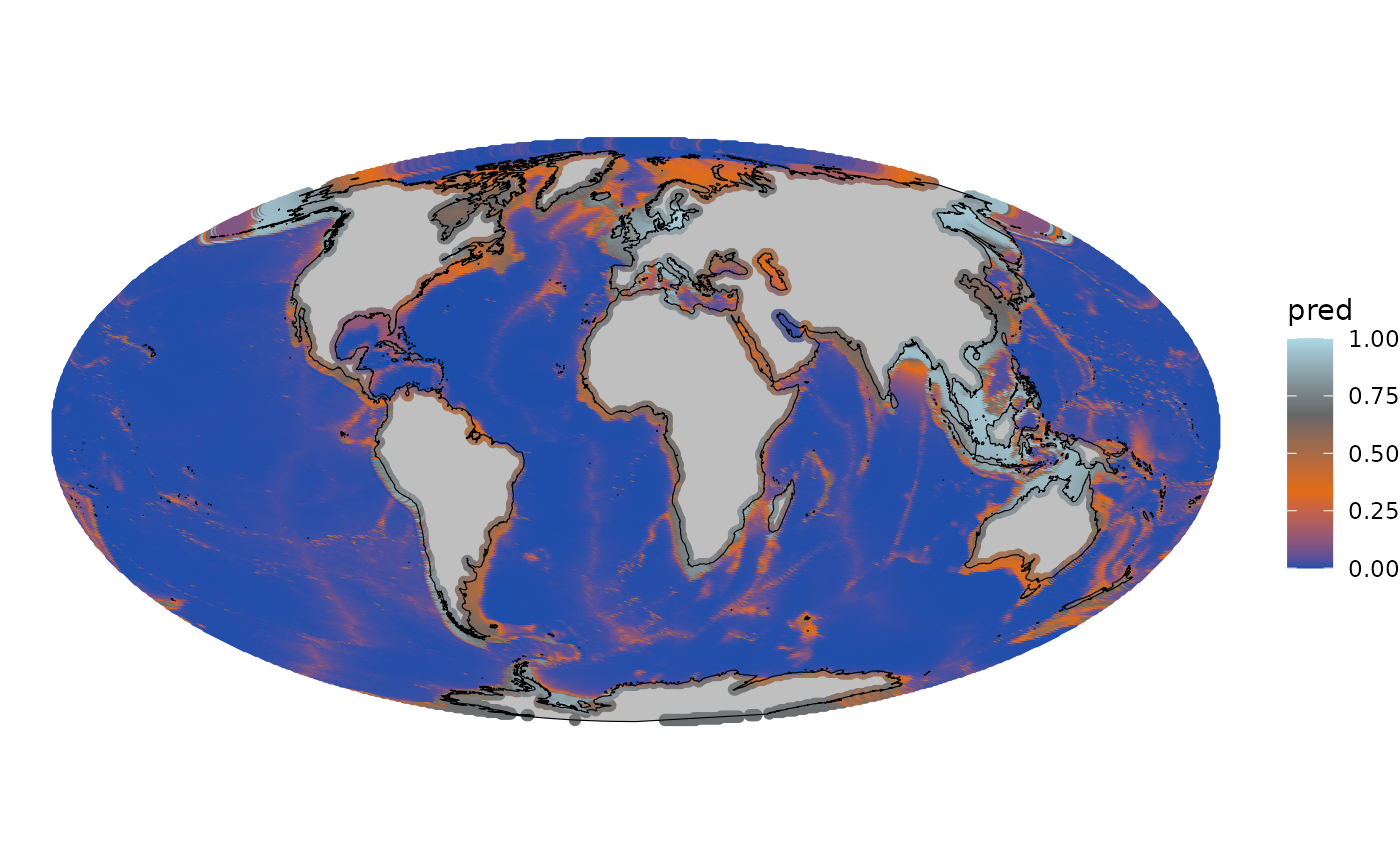
Predicted response variable across the entire domain
Space-time scenarios
After fitting and predicting only in space, we are now going to implement a separable space-time model, as illustrated in Krainski et al., 2018. Essentially, we will include the autoregressive model of order 1 into the spatial effect. As we did with the space examples, we will fit two different likelihoods (Gaussian and Bernoulli). Then, as displayed in the code, we will include an autoregressive term of order 1 with model = “ar1”, where the probability of the parameter being greater than 0 is 0.9.
## Define formula for the space-time effect
rho.prior <- list(prior = 'pc.cor1', param = c(0, 0.9)) ## P(rho>0) = 0.9
form.barrier.st_ar1 <- y ~ 0 + intercept +
  f(beta1, model = "linear") +
  f(i, model = bmodel, group = time,
    control.group = list(model = "ar1",
                         hyper = list(theta = rho.prior)))
Normal response variable
The code for fitting a spatio-temporal scenario is almost the same as in the spatial example; we just include the effect of time in the projector matrix and also in the stack.
## space-time projector matrix
A.st_norm_t <- inla.spde.make.A(
  mesh = smesh,
  loc = cbind(data_model_norm_t$x_coord,
              data_model_norm_t$y_coord,
              data_model_norm_t$z_coord),
  group = data_model_norm_t$time
)

## Stack data for modeling
stk.st_norm_t <- inla.stack(
  data = list(y = data_model_norm_t$y),
  A = list(A.st_norm_t,1,1),
  effects = list(
    list(i = rep(1:bmodel$f$n, k),
         time = rep(1:k, each = bmodel$f$n)),
             beta1 = data_model_norm_t$depth,
    intercept = rep(1, dim(data_model_norm_t)[1])
  )
)
For the fitting, we use the inla function and specify the family as “gaussian” for this particular simulation.
## Fit spatial-temporal model with AR1 correlation structure
result_ar1_norm <- inla(form.barrier.st_ar1,
                   data = inla.stack.data(stk.st_norm_t),
                   family = "gaussian",
                   control.predictor = list(A = inla.stack.A(stk.st_norm_t),
                                            compute = TRUE),
                   control.compute = list(return.marginals.predictor = TRUE),
                   verbose = TRUE)
Then, we can display the main statistical measures for the estimation of the hyperparameters and parameters.
## Print summary of fixed effects
res_summary_fixed_rounded <- round(result_ar1_norm$summary.fixed, 2)
knitr::kable(res_summary_fixed_rounded, caption = "Summary of the posterior distribution of fixed effects.")| mean | sd | 0.025quant | 0.5quant | 0.975quant | mode | kld | |
|---|---|---|---|---|---|---|---|
| intercept | 9.85 | 0.12 | 9.61 | 9.85 | 10.09 | 9.85 | 0 |
| beta1 | -1.50 | 0.00 | -1.51 | -1.50 | -1.50 | -1.50 | 0 |
## Print summary of hyperparameters
res_summary_hyper_rounded <- round(result_ar1_norm$summary.hyperpar, 2)
knitr::kable(res_summary_hyper_rounded, caption = "Summary of the posterior distribution of hyperparameters")| mean | sd | 0.025quant | 0.5quant | 0.975quant | mode | |
|---|---|---|---|---|---|---|
| Precision for the Gaussian observations | 11.15 | 0.13 | 10.90 | 11.15 | 11.41 | 11.14 |
| Theta1 for i | -0.45 | 0.04 | -0.54 | -0.45 | -0.37 | -0.45 |
| Theta2 for i | 0.03 | 0.04 | -0.06 | 0.03 | 0.11 | 0.04 |
| GroupRho for i | 0.98 | 0.00 | 0.98 | 0.98 | 0.98 | 0.98 |
We also compute the marginal distribution for the hyperparameters and parameters, so we can compare the results obtained with the simulated case.
## Plot marginal posterior distributions of hyperparameters
pmarginals <-
  list(
    data.frame(
      param = "range",
      inla.tmarginal(
        function(x) exp(x),
        result_ar1_norm$internal.marginals.hyperpar$`Theta1 for i`)),
    data.frame(
      param = "sigma",
      inla.tmarginal(
        function(x) exp(x),
        result_ar1_norm$internal.marginals.hyperpar$`Theta2 for i`)),
    data.frame(
      param = "sigma_e",
      inla.tmarginal(
        function(x) exp(-x/2),
        result_ar1_norm$internal.marginals.hyperpar$`Log precision for the Gaussian observations`)),
    data.frame(
      param = "rho",
      inla.tmarginal(
        function(x) 1/(1+exp(-x)),
        result_ar1_norm$internal.marginals.hyperpar$`Group rho_intern for i`)),
    data.frame(
      param = "intercept",
      value = result_ar1_norm$marginals.fixed$intercept
    ),
    data.frame(
      param = "beta1",
      value = result_ar1_norm$marginals.fixed$beta1
    )
  )

## Add true values to parameter marginals
pmarginals[[1]]$true <- rep(ranges[1], length(pmarginals[[1]]$x))
pmarginals[[2]]$true <- rep(sigma, length(pmarginals[[1]]$x))
pmarginals[[3]]$true <- rep(sigma_e, length(pmarginals[[1]]$x))
pmarginals[[4]]$true <- rep(rho, length(pmarginals[[1]]$x))
pmarginals[[5]]$true <- rep(beta0_norm, length(pmarginals[[5]]$value.x))
pmarginals[[6]]$true <- rep(beta1_norm, length(pmarginals[[5]]$value.x))
names(pmarginals[[5]]) <- c("param", "x", "y", "true")
names(pmarginals[[6]]) <- c("param", "x", "y", "true")
Parameter and hyperparameters posterior distributions
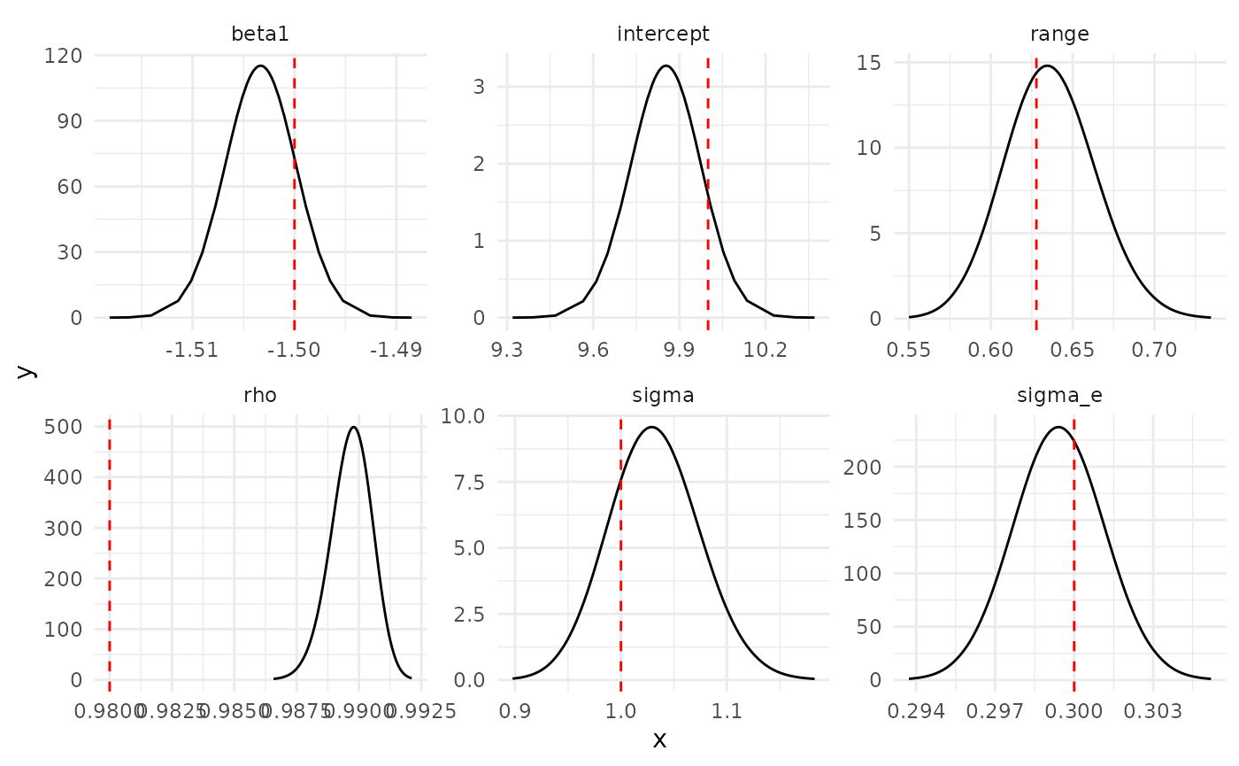
Posterior distribution of parameters and hyperparameters, where, beta1 represents the coefficient for the depth covariate, rho represents the correlation parameter for the autoregressive model of order 1, sigma represents the standard deviation of the random field, and sigma.e represents the standard deviation of the Gaussian distribution.
Bernouilli response variable
The same framework as that for the Normal response variable can be applied to the Bernoulli response variable. We simply need to change the family in the inla function to “binomial”. Consequently, we obtain similar outputs, but in this case, they parameter of interest is a probability.
## space-time projector matrix
A.st_ber_t <- inla.spde.make.A(
  mesh = smesh,
  loc = cbind(data_model_ber_t$x_coord,
              data_model_ber_t$y_coord,
              data_model_ber_t$z_coord),
  group = data_model_ber_t$time
)

## Stack data for modeling
stk.st_ber_t <- inla.stack(
  data = list(y = data_model_ber_t$y),
  A = list(A.st_ber_t,1,1),
  effects = list(
    list(i = rep(1:bmodel$f$n, k),
         time = rep(1:k, each = bmodel$f$n)),
             beta1 = data_model_ber_t$depth,
    intercept = rep(1, dim(data_model_ber_t)[1])
  )
)

## Define formula for the space-time effect
rho.prior <- list(prior = 'pc.cor1', param = c(0, 0.9)) ### P(rho>0) = 0.9
form.barrier.st_ar1 <- y ~ 0 + intercept +
  f(beta1, model = "linear") +
  f(i, model = bmodel, group = time,
    control.group = list(model = "ar1",
                         hyper = list(theta = rho.prior)))

## Fit spatial-temporal model with AR1 correlation structure
result_ar1_ber <- inla(form.barrier.st_ar1,
                   data = inla.stack.data(stk.st_ber_t),
                   family = "binomial",
                   control.predictor = list(A = inla.stack.A(stk.st_ber_t),
                                            compute = TRUE),
                   control.compute = list(return.marginals.predictor = TRUE),
                   verbose = TRUE)

## Print summary of fixed effects
res_summary_fixed_rounded <- round(result_ar1_ber$summary.fixed, 2)
knitr::kable(res_summary_fixed_rounded, caption = "Summary of the posterior distribution of fixed effects.")| mean | sd | 0.025quant | 0.5quant | 0.975quant | mode | kld | |
|---|---|---|---|---|---|---|---|
| intercept | 0.77 | 0.37 | -0.02 | 0.79 | 1.44 | 0.85 | 0 |
| beta1 | -1.43 | 0.04 | -1.50 | -1.43 | -1.36 | -1.43 | 0 |
## Print summary of hyperparameters
res_summary_hyper_rounded <- round(result_ar1_ber$summary.hyperpar, 2)
knitr::kable(res_summary_hyper_rounded, caption = "Summary of the posterior distribution of hyperparameters")| mean | sd | 0.025quant | 0.5quant | 0.975quant | mode | |
|---|---|---|---|---|---|---|
| Theta1 for i | -0.14 | 0.16 | -0.45 | -0.14 | 0.19 | -0.15 |
| Theta2 for i | 0.11 | 0.10 | -0.09 | 0.11 | 0.31 | 0.10 |
| GroupRho for i | 0.99 | 0.01 | 0.96 | 0.99 | 1.00 | 0.99 |
## Plot marginal posterior distributions of hyperparameters
pmarginals <-
  list(
    data.frame(
      param = "range",
      inla.tmarginal(
        function(x) exp(x),
        result_ar1_ber$internal.marginals.hyperpar$`Theta1 for i`)),
    data.frame(
      param = "sigma",
      inla.tmarginal(
        function(x) exp(x),
        result_ar1_ber$internal.marginals.hyperpar$`Theta2 for i`)),
    data.frame(
      param = "rho",
      inla.tmarginal(
        function(x) 1/(1+exp(-x)),
        result_ar1_ber$internal.marginals.hyperpar$`Group rho_intern for i`)),
    data.frame(
      param = "intercept",
      value = result_ar1_ber$marginals.fixed$intercept
    ),
    data.frame(
      param = "beta1",
      value = result_ar1_ber$marginals.fixed$beta1
    )
  )

## Add true values to parameter marginals
pmarginals[[1]]$true <- rep(ranges[1], length(pmarginals[[1]]$x))
pmarginals[[2]]$true <- rep(sigma, length(pmarginals[[1]]$x))
pmarginals[[3]]$true <- rep(rho, length(pmarginals[[1]]$x))
pmarginals[[4]]$true <- rep(beta0_ber, length(pmarginals[[4]]$value.x))
pmarginals[[5]]$true <- rep(beta1_ber, length(pmarginals[[5]]$value.x))
names(pmarginals[[4]]) <- c("param", "x", "y", "true")
names(pmarginals[[5]]) <- c("param", "x", "y", "true")
Parameter and hyperparameters posterior distributions
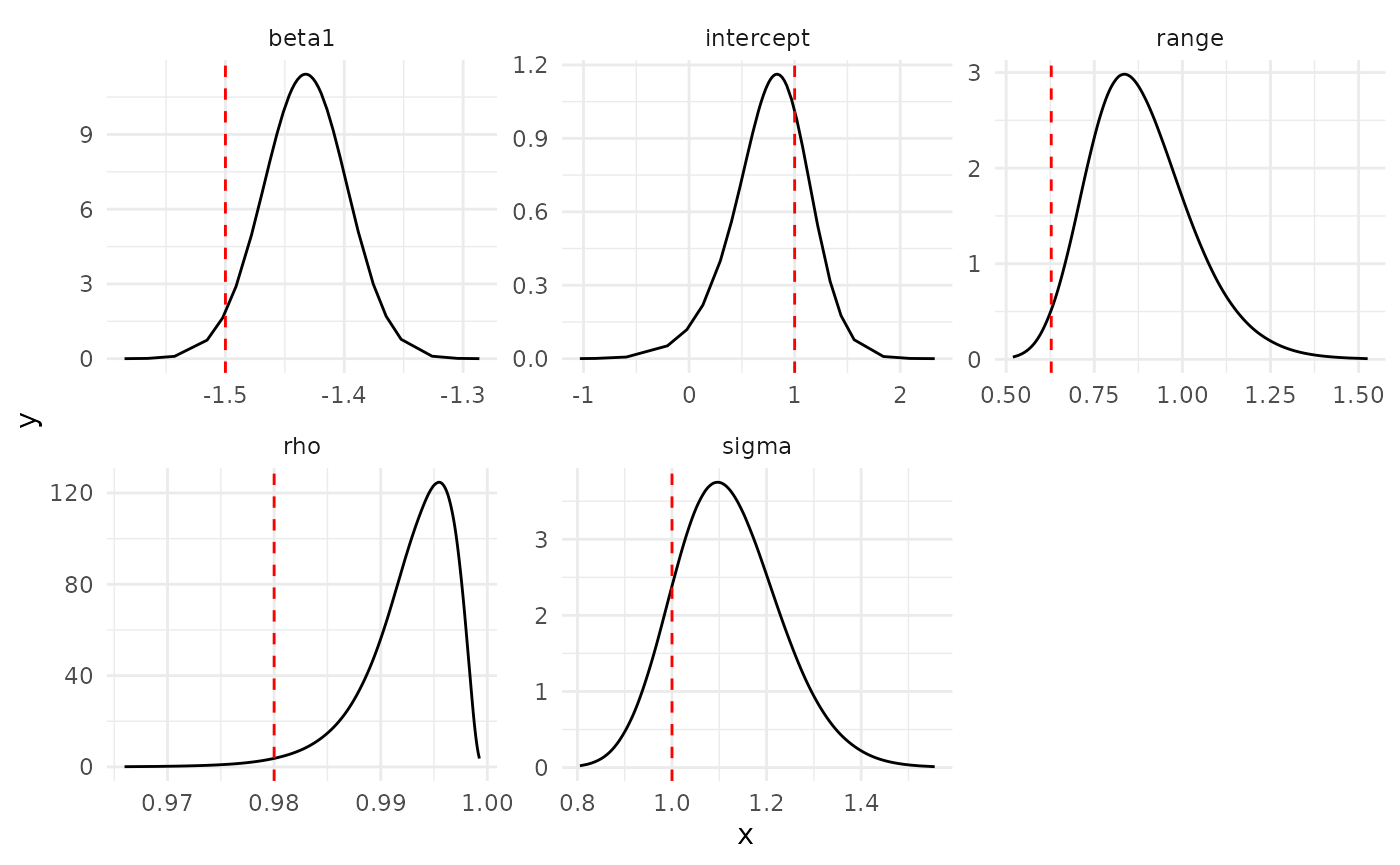
Posterior distribution of parameters and hyperparameters, where, beta1 represents the coefficient for the depth covariate, rho represents the correlation parameter for the autoregressive model of order 1, and sigma represents the standar deviation of the random field.
Session information
## R version 4.5.3 (2026-03-11)
## Platform: x86_64-pc-linux-gnu
## Running under: Ubuntu 24.04.4 LTS
##
## Matrix products: default
## BLAS:   /usr/lib/x86_64-linux-gnu/openblas-pthread/libblas.so.3
## LAPACK: /usr/lib/x86_64-linux-gnu/openblas-pthread/libopenblasp-r0.3.26.so;  LAPACK version 3.12.0
##
## locale:
##  [1] LC_CTYPE=C.UTF-8       LC_NUMERIC=C           LC_TIME=C.UTF-8
##  [4] LC_COLLATE=C.UTF-8     LC_MONETARY=C.UTF-8    LC_MESSAGES=C.UTF-8
##  [7] LC_PAPER=C.UTF-8       LC_NAME=C              LC_ADDRESS=C
## [10] LC_TELEPHONE=C         LC_MEASUREMENT=C.UTF-8 LC_IDENTIFICATION=C
##
## time zone: UTC
## tzcode source: system (glibc)
##
## attached base packages:
## [1] stats     graphics  grDevices utils     datasets  methods   base
##
## other attached packages:
##  [1] ggpubr_0.6.3             DOYPAColors_0.0.2        s2_1.1.9
##  [4] ggOceanMaps_2.3.0        inlabru_2.14.0           fmesher_0.7.0
##  [7] INLAspacetime_0.1.13.905 ggplot2_4.0.2            sf_1.1-0
## [10] rnaturalearth_1.2.0      rmarkdown_2.31           knitr_1.51
## [13] INLA_26.03.19            Matrix_1.7-4
##
## loaded via a namespace (and not attached):
##  [1] gtable_0.3.6            xfun_0.57               bslib_0.10.0
##  [4] rstatix_0.7.3           lattice_0.22-9          vctrs_0.7.2
##  [7] tools_4.5.3             generics_0.1.4          spdep_1.4-2
## [10] parallel_4.5.3          tibble_3.3.1            proxy_0.4-29
## [13] pkgconfig_2.0.3         INLAtools_0.1.2         KernSmooth_2.23-26
## [16] RColorBrewer_1.1-3      S7_0.2.1                desc_1.4.3
## [19] lifecycle_1.0.5         deldir_2.0-4            compiler_4.5.3
## [22] farver_2.1.2            MatrixModels_0.5-4      textshaping_1.0.5
## [25] carData_3.0-6           stars_0.7-2             htmltools_0.5.9
## [28] class_7.3-23            sass_0.4.10             yaml_2.3.12
## [31] Formula_1.2-5           car_3.1-5               tidyr_1.3.2
## [34] pillar_1.11.1           pkgdown_2.2.0           jquerylib_0.1.4
## [37] classInt_0.4-11         cachem_1.1.0            wk_0.9.5
## [40] boot_1.3-32             abind_1.4-8             rnaturalearthdata_1.0.0
## [43] Deriv_4.2.0             tidyselect_1.2.1        digest_0.6.39
## [46] dplyr_1.2.1             purrr_1.2.1             labeling_0.4.3
## [49] splines_4.5.3           cowplot_1.2.0           fastmap_1.2.0
## [52] grid_4.5.3              cli_3.6.6               magrittr_2.0.5
## [55] broom_1.0.12            e1071_1.7-17            withr_3.0.2
## [58] backports_1.5.1         scales_1.4.0            sp_2.2-1
## [61] spData_2.3.4            gridExtra_2.3           ggsignif_0.6.4
## [64] ragg_1.5.2              evaluate_1.0.5          rlang_1.2.0
## [67] Rcpp_1.1.1              glue_1.8.0              DBI_1.3.0
## [70] jsonlite_2.0.0          plyr_1.8.9              R6_2.6.1
## [73] systemfonts_1.3.2       fs_2.0.1                units_1.0-1
References
Bakka, H., J. Vanhatalo, J. Illian, D. Simpson, and H. Rue. 2019. “Non-Stationary Gaussian Models with Physical Barriers.” Spatial Statistics 29 (March): 268–88. https://doi.org/https://doi.org/10.1016/j.spasta.2019.01.002.
Lindgren, Finn, Håvard Rue, and Johan Lindström. 2011. “An Explicit Link Between Gaussian Fields and Gaussian Markov Random Fields: The Stochastic Partial Differential Equation Approach.” Journal of the Royal Statistical Society: Series B (Statistical Methodology) 73 (4): 423–98. https://doi.org/10.1111/j.1467-9868.2011.00777.x.
Krainski, E., Gómez-Rubio, V., Bakka, H., Lenzi, A., Castro-Camilo, D., Simpson, D., Lindgren, F. and Rue, H. (2018). Advanced spatial modeling with stochastic partial differential equations using R and INLA. Chapman and Hall/CRC.
